Help with Multivariate SDE Timeseries

I may have found a way to workaround the problem but am getting errors. I defined \epsilon_t^s b using pm.Normal like before. I pass this into the drift coefficient of the variance process SDE, as before. For the return process, I can’t use pm.Deterministic because I can’t pass in the observed returns. But what if I specify the return process as an SDE with 1) \epsilon_t^s passed into the drift coefficient and 2) a zero diffusion coefficient?

import numpy as np
import matplotlib.pyplot as plt
import pymc3 as pm
from pymc3.distributions.timeseries import EulerMaruyama

returns = np.genfromtxt(pm.get_data("SP500.csv"))

def Vt_sde(Vt, sigma_v, rho, beta_v, alpha_v, error_s):
    return alpha_v + beta_v * Vt + sigma_v * np.sqrt(Vt) * rho * error_s, sigma_v * np.sqrt(Vt) * np.sqrt(1-rho*rho)

def Yt_sde(Vt, error_s):
    return np.sqrt(Vt) * error_s,0

with pm.Model() as sp500_model:

    alpha_v=pm.Normal('alpha',0,sd=100)
    beta_v=pm.Normal('beta',0,sd=10)
    sigma_v=pm.InverseGamma('sigmaV',2.5,0.1)
    rho=pm.Uniform('rho',-.9,.9)

    error_s = pm.Normal('error_s',mu=0.0,sd=1)
    Vt = EulerMaruyama('Vt', 1.0, Vt_sde, [sigma_v, rho, alpha_v, beta_v, error_s], shape=len(returns),testval=np.repeat(.01,len(returns)))
    Yt = EulerMaruyama('Yt', 1.0,Yt_sde, [Vt, error_s], observed=returns)
        

Unfortunately I am getting the following error…

TypeError: Yt_sde() takes 2 positional arguments but 3 were given

I’m not sure how pm.Potential would help here. I can’t pass an observed variable into pm.Potential

Is there a reason why pm.Deterministic does not allow you to pass in an observed variable? Are there any workarounds?

This might work. I can work out the log probability of the posterior for this problem, which I can implement as class similar to MVGuassianRandomWalk. How would I implement an example like what you’ve described for a simple MvGuassianRandomWalk?

Thanks everyone for the help I really hope I can get this model implemented somehow!

Any help on this? I’m at a dead end.

pymc3 needs a likelihood function to sample, and if you observed a function of some random variables (ie., observing a Deterministic) the likelihood expression is not trivial. Workaround is using a normal distribution with the deterministic output as mu and a small sd (.1 - 1) and observed=data.

So you can first do s_data = theano.shared(data), and then after you write down your model, you use theano.tensor.stack or theano.tensor.concatenate to concatenate the latent observed with s_data and feed it to MvGuassianRandomWalk.

I tried implementing the model without correlation as a starting point but am getting a “Bad Initial Energy” error. I tried setting init=‘adapt_diag’ in pm.sample but still get the error. I even tried changing my priors to ensure they are positive.


import numpy as np
import matplotlib.pyplot as plt
import pymc3 as pm
from pymc3.distributions.timeseries import EulerMaruyama

returns = np.genfromtxt(pm.get_data("SP500.csv"))

def Vt_sde(Vt, sigmaV, kappa, theta):
    return kappa*(theta-Vt), sigmaV *np.sqrt(Vt)

with pm.Model() as sp500_model:

    theta=pm.HalfNormal('theta',sd=0.4)
    kappa=pm.HalfNormal('kappa',sd=2)
    sigmaV=pm.InverseGamma('sigmaV',2.5,0.1)
    
    Vt = EulerMaruyama('Vt',1.0,Vt_sde,[sigmaV, kappa, theta],shape=len(returns),testval=np.repeat(.01,len(returns)))
    volatility_process = pm.Deterministic('volatility_process', np.sqrt(Vt))
    r = pm.Normal('r', mu=0,sd=volatility_process, observed=returns)
    
with sp500_model:
    trace = pm.sample(2000,chains=1,cores=1)
    
pm.traceplot(trace, [sigmaV, kappa, theta],init='adapt_diag');

ValueError: Bad initial energy: inf. The model might be misspecified.

Ok I think I solved that issue…need to ensure Vt is positive when taking the square root. Now I just need to get the correlation worked in

import numpy as np
import matplotlib.pyplot as plt
import pymc3 as pm
from pymc3.distributions.timeseries import EulerMaruyama

returns = np.genfromtxt(pm.get_data("SP500.csv"))

def Vt_sde(Vt, sigmaV, kappa, theta):
    return kappa*(theta-Vt), sigmaV *np.sqrt(np.abs(Vt))

with pm.Model() as sp500_model:

    theta=pm.HalfNormal('theta',sd=0.4)
    kappa=pm.HalfNormal('kappa',sd=2)
    sigmaV=pm.InverseGamma('sigmaV',2.5,0.1)
    
    Vt = EulerMaruyama('Vt',1.0,Vt_sde,[sigmaV, kappa, theta],shape=len(returns),testval=np.repeat(.01,len(returns)))
    volatility_process = pm.Deterministic('volatility_process', np.sqrt(np.abs(Vt)))
    r = pm.Normal('r', mu=0,sd=volatility_process, observed=returns)
    
with sp500_model:
    trace = pm.sample(2000,chains=1,cores=1)
    
pm.traceplot(trace, [sigmaV, kappa, theta])

Even with that fix, the output doesn’t make any sense.

Well, since I cant get this model working even when the volatility process is independent, perhaps we can try a model that does work. This is a similar model but instead of variance being stochastic, log-variance follows an AR(1) process:

Y_t are the observed returns and V_t the latend variance process
Y_t=\sqrt{V_{t-1}}\epsilon_t^s
log(V_t)=\alpha_v+\beta_vlog(V_{t-1})+\sigma_v\epsilon_t^v

For independent epsilon, implementation is straightforward. The log-variance process can implemented either using the AR class or EurlerMaruyama.


import numpy as np
import matplotlib.pyplot as plt
import pymc3 as pm
from pymc3.distributions.timeseries import EulerMaruyama

returns = np.genfromtxt(pm.get_data("SP500.csv"))

def logV_sde(logV, sigmaV, beta, alpha):
    return alpha + beta * logV, sigmaV 

with pm.Model() as sp500_model:

    alpha=pm.Normal('alpha',0,sd=100)
    beta=pm.Normal('beta',0,sd=10)
    sigmaV=pm.InverseGamma('sigmaV',2.5,0.1)
    
    logV = pm.AR('logV', [alpha,beta], sd=sigmaV**.5,constant=True,shape=len(returns))
    #logV = EulerMaruyama('logV',1.0,logV_sde,[sigmaV, beta, alpha],shape=len(returns),testval=np.repeat(.01,len(returns)))
    volatility_process = pm.Deterministic('volatility_process', pm.math.exp(.5*logV))
    r = pm.Normal('r', mu=0,sd=volatility_process, observed=returns)
    
with sp500_model:
    trace = pm.sample(2000,chains=1,cores=1)
    
pm.traceplot(trace, [alpha,beta,sigmaV]);
    

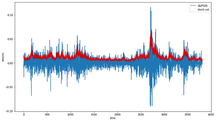
fig, ax = plt.subplots(figsize=(14, 8))
ax.plot(returns)
ax.plot(trace['volatility_process',::5].T, 'r', alpha=.03);
ax.set(xlabel='time', ylabel='returns')
ax.legend(['S&P500', 'stoch vol']);

the results make sense, and the volatility trace is similar to what we see in the PyMC3 stochastic volatility example:

Using this model as starting point, I’d like to introduce a correlation \rho between \epsilon_t^s and \epsilon_t^v . I’ve tried a workaround discussed earlier in this thread but the introduction of a third random variable produces nonsensical results. I think the proper solution is define the multivariate posterior and pass in the observed returns. This I don’t know how to do

1 Like

Oh yes I remember @twiecki mentioned somewhere that if you have double stochastic (i.e., random walk of variance plus random walk of mean) it is extremely difficult to do inference.

1 Like

I don’t think this particular problem is that difficult, it can be done using Metropolis but it tends to be slow. I think NUTS can handle it if we specify the model correctly.

Here’s how I think we could set up the model:

  • Create a new timeseries class similar to MVGuassianRandomWalk
  • Modify the logp function to accommodate the bivariate posterior of Y and V. In the example of the log-vol model above, the logvol follows an AR1 process so the code will look similar to the AR1 class
  • Once the logp function is defined correctly, pass in the observed return series concatenated with the latent state

Alternatively, we can take the approach outlined in this paper


In section 2.3 the authors consider the same log-vol model with correlated errors and adopt a Metropolis scheme

Here’s a possible workaround…though I still prefer the type of solution involving a new multivariate class…

is it possible to define a Deterministic that’s a recursive function? this would be similar to the vol-update function in the GARCH class.

Consider the model again:
Y_t=\sqrt{V_{t-1}}\epsilon_t^s
log(V_t)=\alpha_v+\beta_vlog(V_{t-1})+\sigma_v\epsilon_t^v
\epsilon_t^s and \epsilon_t^v have correlation \rho

Set \epsilon^s=\rho\epsilon_t^v+\sqrt{1-\rho^2}\epsilon_t^n so that \epsilon_t^v and \epsilon_t^n are independent standard normals. Then we have
Y_t=\sqrt{V_{t-1}}[\rho\epsilon_t^v+\sqrt{1-\rho^2}\epsilon_t^n]
log(V_t)=\alpha_v+\beta_vlog(V_{t-1})+\sigma_v\epsilon_t^v

Now I can set up the model as follows

alpha=pm.Normal('alpha',0,sd=100)
beta=pm.Normal('beta',0,sd=10)
sigma_v=pm.InverseGamma('sigma_v',2.5,0.1)
epsilon_v=pm.Normal('error_v',mu=0,sd=1)

logV(t) is now a deterministic function of epsilon_v and the priors, but is recursive since it also depends on logV(t-1) this is the missing step

volatility=pm.Deterministic('volatility', pm.math.exp(.5*logV))
Yt=pm.Normal('Yt',mu=volatility*rho*error_v,sd=volatility*np.sqrt(1-rho*rho),observed=returns)

would something like this work?

I think I was able to implement the workaround, but the sampling is extremely slow.


import numpy as np
import matplotlib.pyplot as plt
import pymc3 as pm
from pymc3.distributions.timeseries import EulerMaruyama
import theano.tensor as tt
from theano import scan

returns = np.genfromtxt(pm.get_data("SP500.csv"))

def get_volatility(x,initial_vol,alpha,beta,sigma):
    x = x[:-1]

    def volatility_update(x, vol, a, b,sigma):
        return a + beta * vol + sigma * x

    vol, _ = scan(fn=volatility_update,
                  sequences=[x],
                  outputs_info=[initial_vol],
                  non_sequences=[alpha, beta,
                                 sigma])
    return tt.concatenate([[initial_vol], vol])


with pm.Model() as sp500_model:

    alpha=pm.Normal('alpha',0,sd=100)
    beta=pm.Normal('beta',0,sd=10)
    sigma_v=pm.InverseGamma('sigma_v',2.5,0.1)
    error_v=pm.Normal('error_v',mu=0,sd=1,shape=len(returns))
    rho=pm.Uniform('rho',-.9,.9)


    logV=get_volatility(error_v,.01,alpha,beta,sigma_v)

    volatility_process = pm.Deterministic('volatility_process', pm.math.exp(.5*logV))
    r=pm.Normal('r',mu=volatility_process*rho*error_v,sd=volatility_process*np.sqrt(1-rho*rho),observed=returns)


with sp500_model:
    trace = pm.sample(2000,chains=1,cores=1)

pm.traceplot(trace, [alpha,beta,sigma_v]);
    
fig, ax = plt.subplots(figsize=(14, 8))
ax.plot(returns)
ax.plot(trace['volatility_process',::5].T, 'r', alpha=.03);
ax.set(xlabel='time', ylabel='returns')
ax.legend(['S&P500', 'stoch vol']);

2 Likes

Were you ever able to get this code up and running? the thread ended without a known solution

No, not within PyMC3.

1 Like

Did you make it work with another package? Would be interested to hear how it went.

Regarding @jungpenglao 's comment that it’s not trivial to allow observed Deterministic variables, what’s the blocker?

Say we observe \tilde{x}_i = f(x, a), where x \sim N(0, b^2), a and b are stochastic variables and \tilde{x} is the observed variable. If we invert f we can write f^{-1}(\tilde{x}_i, a) \sim N(0, b^2). Given values for a and b we could calculate the likelihood easily, and also its partial derivatives with a and b (or am I missing something).

So is it possible to enter a Deterministic variable as the observed value of a stochastic variable? I might be missing something here.

When f is easy to work with and can be automatically inverted, then perhaps that’s the case. There are many situations where it’s not feasible to invert f (or even tell if f is invertible to begin with), so getting a general purpose solution to this is out of reach at the moment.

Sorry for the bothering. I am working on Heston model now, but fail to get the result. Did you come up with a solution finally? Thanks in advance.