I might take a Poisson Process approach to these data; denoting by
r_t^{(i)}
the instantaneous tweet rate for hashtag i. Then the number of observed tweets in a given period looks like
N(t_b, t_e) \sim \mathrm{Pois}(r_{b,e}) \;\;\; r_{b,e} = \int_{t_b}^{t_e} r_t dt
You’ve got a resolution of 1 minute (maybe 1 second); so in that case you’d have
N_t^{(i)} \sim \mathrm{Pois}(r_t^{(i)})
for the tth minute (or second?) and ith hashtag. Under this framework, the modeling all has to do with functional terms you introduce into r_t, such as \cos(60 \pi t) for hourly effects. Just to play around:
import pymc3 as pm
import numpy as np
import theano
import theano.tensor as tt
from matplotlib import pyplot as plt

# let a "tick" be one second
DAYS=7
SEC_MIN=60
MIN_HR=60
HR_DAY=24

N_TICK = DAYS*HR_DAY*MIN_HR*SEC_MIN


# 2 / day * (1 day / 24 H) * (1 H / 60 min)

HALF_DAILY_FREQ = 4./(HR_DAY*MIN_HR*SEC_MIN)
DAILY_FREQ = HALF_DAILY_FREQ/2

HOURLY_PHASES = SEC_MIN*MIN_HR*np.arange(24, dtype=np.float32)/(HR_DAY*MIN_HR*SEC_MIN)

ALPHAS = [0.]*24

ALPHAS[20] = 1e-3
alpha_happy_hour = 5e-1

base_rate = 3e-3

time_index = np.arange(N_TICK)
with pm.Model() as mod:
    rate_noise = pm.Normal('noise', 0, base_rate/2., shape=N_TICK)
    rate = np.log(base_rate) + rate_noise
    for i in range(len(ALPHAS)):
        test_fx = tt.cos(np.pi * (HALF_DAILY_FREQ * time_index + HOURLY_PHASES[i]))
        rate = rate + test_fx * ALPHAS[i]
    # happy hour phase
    test_fx = tt.cos(np.pi* (DAILY_FREQ* time_index + HOURLY_PHASES[17]))
    rate = rate + test_fx * alpha_happy_hour
    rate = pm.Deterministic('rate', tt.exp(rate))
    tweets = pm.Poisson('tweets', rate, shape=N_TICK)
    runs = pm.sample_prior_predictive(25)

plt.plot(runs['rate'][0,:]);
midnights = np.arange(DAYS)*HR_DAY*MIN_HR*SEC_MIN
noons = (0.5 + np.arange(DAYS))*HR_DAY*MIN_HR*SEC_MIN
for m in midnights:
    plt.plot([m, m], [-1, 1], 'k-')
for n in noons:
    plt.plot([n, n], [-1, 1], 'b-')
mn = np.min(runs['rate'][0,:])
mx = np.max(runs['rate'][0,:])
plt.ylim([mn, mx])
plt.figure();
plt.plot(runs['tweets'][0,:50000]);


From this it should be clear that in this model the sub-hourly effects are just noise and average out – and also that the hourly effects (by virtue of being periodic) also average out to the daily level.
import itertools
def hourfx(t):
    return int(t[1]/(SEC_MIN*MIN_HR))

def dayfx(t):
    return int(t[1]/(SEC_MIN*MIN_HR*HR_DAY))

hourly_tweets = itertools.groupby(zip(runs['tweets'][0,:], time_index), hourfx)
hourly_tweets = [np.sum([x[0] for x in v]) for k, v in hourly_tweets]

daily_tweets = itertools.groupby(zip(runs['tweets'][0,:], time_index), dayfx)
daily_tweets = [np.sum([x[0] for x in v]) for k, v in daily_tweets]

plt.plot(hourly_tweets)
plt.plot(daily_tweets)


One can start introducing test functions just as in a linear model:
days = DAYS
hours_day = HR_DAY

want_freqs = [1./hours_day]
want_phase = np.array([4., 15., 22.])/hours_day

time_index = np.arange(days*hours_day)
with pm.Model() as hourly_model:
    log_base_rate = pm.Normal('base_rate_log', -3, 3.)
    rate = log_base_rate
    for i, f in enumerate(want_freqs):
        for j, p in enumerate(want_phase):
            test_alpha = pm.Laplace('alpha_{}_{}'.format(i, j), 0., 1.)
            test_fx = tt.cos(2*np.pi * (want_freqs[i]*time_index + want_phase[j]))
            rate = rate + test_alpha*test_fx
    #erate = pm.Deterministic('log_rate', rate)
    tweets = pm.Poisson('hourly_tweets', tt.exp(rate), observed=np.array(hourly_tweets))
    trace = pm.sample(600, chains=5, init='jitter+adapt_diag')
pm.traceplot(trace)
And looking at the posterior:
with hourly_model:
    post = pm.sample_posterior_predictive(trace)


median_tweets = np.median(post['hourly_tweets'], axis=0)
u90_tweets = np.percentile(post['hourly_tweets'], 95, axis=0)
l90_tweets = np.percentile(post['hourly_tweets'], 5, axis=0)

plt.plot(median_tweets)
plt.plot(u90_tweets, 'grey')
plt.plot(l90_tweets, 'grey')
plt.plot(hourly_tweets, 'red', alpha=0.5)

Additionally, one can introduce lags and differences such as
L_k r_t = r_{t-k}
\Delta r_t = r_t - r_{t-1} = r_t - L_1r_t
and make the rate of the next step depend on the number of tweets observed:
l1 = np.array([0] + hourly_tweets[1:])
l2 = np.array([0, 0] + hourly_tweets[2:])
l3 = np.array([0, 0, 0] + hourly_tweets[3:])
l4 = np.array([0, 0, 0, 0] + hourly_tweets[4:])
with pm.Model() as lagged_hourly:
log_base_rate = pm.Normal('base_rate_log', -3, 3.)
rate = log_base_rate
a1 = pm.Normal('a1', 0., 1.)
a2 = pm.Normal('a2', 0., 1.)
a3 = pm.Normal('a3', 0., 1.)
a4 = pm.Normal('a4', 0., 1.)
rate = rate + a1 * np.log(1 + l1) + a2 * np.log(1 + l2) + a3 * np.log(1 + l3) + a4 * np.log(1 + l4)
tweets = pm.Poisson('hourly_tweets', tt.exp(rate), observed=np.array(hourly_tweets))
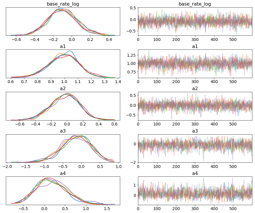
trace2 = pm.sample(600, chains=5, init='jitter+adapt_diag')
pm.traceplot(trace2);
with lagged_hourly:
post = pm.sample_posterior_predictive(trace2)
median_tweets = np.median(post['hourly_tweets'], axis=0)
u90_tweets = np.percentile(post['hourly_tweets'], 95, axis=0)
l90_tweets = np.percentile(post['hourly_tweets'], 5, axis=0)
plt.plot(median_tweets)
plt.plot(u90_tweets, 'grey')
plt.plot(l90_tweets, 'grey')
plt.plot(hourly_tweets, 'red', alpha=0.5)