Unique solution for probabilistic PCA

@ferrine

I got the model to report average loss properly by changing w in symbolic_logp_not_scaled from [.5,.5] to theano.tensor.stack([.5,.5]).

@node_property
def symbolic_logq_not_scaled(self):

    z = self.symbolic_random
    
    mu=theano.tensor.stack([self.mean, -self.mean])
    sd=theano.tensor.stack([self.std, self.std])
                           
    logq = NormalMixture.dist(w=theano.tensor.stack([.5,.5]), 
                                 mu=mu, 
                                 sd=sd
                                ).logp(z)
    
    return logq.sum(range(1, logq.ndim))

My SMF implementation that I used in my experiments
IMPORTANT!

# if we sample from mixture, we should not broadcast random sign!!!
# this works with 1 sample approximationm but it does not matter here
sign = pm.floatX(theano.tensor.as_tensor([-1, 1]))[(self._rng.uniform(()) > 0).astype('int8')]
from pymc3.variational.opvi import Group, node_property
from pymc3.variational.approximations import MeanFieldGroup

@Group.register
class SymmetricMeanFieldGroup(MeanFieldGroup):
    """Symmetric MeanField Group for Symmetrized VI"""
    __param_spec__ = dict(smu=('d', ), rho=('d', ))
    short_name = 'sym_mean_field'
    alias_names = frozenset(['smf'])
    
    @node_property
    def mean(self):
        return self.params_dict['smu']

    def create_shared_params(self, start=None):
        if start is None:
            start = self.model.test_point
        else:
            start_ = start.copy()
            update_start_vals(start_, self.model.test_point, self.model)
            start = start_
        if self.batched:
            start = start[self.group[0].name][0]
        else:
            start = self.bij.map(start)
        rho = np.zeros((self.ddim,))
        if self.batched:
            start = np.tile(start, (self.bdim, 1))
            rho = np.tile(rho, (self.bdim, 1))
        return {'smu': theano.shared(
                    pm.floatX(start), 'smu'),
                'rho': theano.shared(
                    pm.floatX(rho), 'rho')}
    
    @node_property
    def symbolic_random(self):
        initial = self.symbolic_initial
        # if we sample from mixture, we should not broadcast random sign!!!
        sign = pm.floatX(theano.tensor.as_tensor([-1, 1]))[(self._rng.uniform(()) > 0).astype('int8')]
        sigma = self.std
        mu = self.mean
        return sigma * initial + mu * sign

    @node_property
    def symbolic_logq_not_scaled(self):
        z = self.symbolic_random
        sigma = self.std
        mu = self.mean
        logq = .5 * (
            pm.Normal.dist(mu=mu, sd=sigma).logp(z)
            +
            pm.Normal.dist(mu=-mu, sd=sigma).logp(z)
        )    
        return logq.sum(range(1, logq.ndim))

Code to setup inference

with model1:
    symmetric_group = pm.Group([w], vfam='smf')
    other_group = pm.Group(None, vfam='mf')
    approx = pm.Approximation([symmetric_group, other_group])
    inference = pm.KLqp(approx)

optional starting point

symmetric_group.params_dict['smu'].set_value(np.ones(symmetric_group.ddim, dtype='float32'))
# rho (sigma=softplus(rho)) parametrization
symmetric_group.params_dict['rho'].set_value(np.ones(symmetric_group.ddim, dtype='float32'))

Running inference

inference.fit(25000)


image

Strange things happen, I have loss going to undefined regions(( IUnfortunately not much time to investigate

1 Like

@ferrine

The model is working correctly for me as described before, (without change to symbolic_random).

Now the only thing I’m working on is getting Minibatch to work.
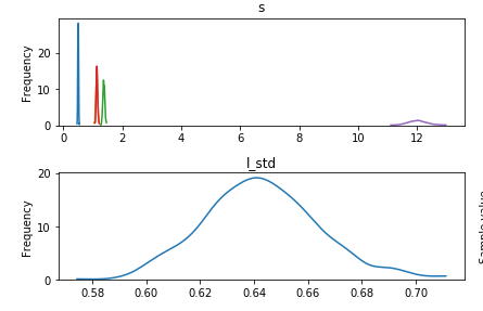
Here are the weights traceplot from the full dataset
image

While the weights from the Minibatch dataset are very similar, their sds are higher, and the cov parameter is underestimated. (the resulting correlation matrix is almost all 0)
image

To clarify, here’s the code I’m working with:

class NormalMixture(pm.Mixture):
    def __init__(self, w, mu, comp_shape=(), *args, **kwargs):
        sd=kwargs.pop('sd',None)
        self.mu = mu = tt.as_tensor_variable(mu)
        self.sd = sd = tt.as_tensor_variable(sd)

        super(NormalMixture, self).__init__(w, [pm.Normal.dist(mu[0], sd=sd[0]),pm.Normal.dist(mu[1], sd=sd[1])],
                                            *args, **kwargs)

    def _repr_latex_(self, name=None, dist=None):
        if dist is None:
            dist = self
        mu = dist.mu
        w = dist.w
        sd = dist.sd
        name = r'\text{%s}' % name
        return r'${} \sim \text{{NormalMixture}}(\mathit{{w}}={},~\mathit{{mu}}={},~\mathit{{sigma}}={})$'.format(name,
                                                get_variable_name(w),
                                                get_variable_name(mu),
                                                get_variable_name(sd))

@Group.register
class SymmetricMeanFieldGroup(MeanFieldGroup):
    """Symmetric MeanField Group for Symmetrized VI"""
    __param_spec__ = dict(smu=('d', ), rho=('d', ))
    short_name = 'sym_mean_field'
    alias_names = frozenset(['smf'])
    
    @node_property
    def mean(self):
        return self.params_dict['smu']

    def create_shared_params(self, start=None):
        if start is None:
            start = self.model.test_point
        else:
            start_ = start.copy()
            update_start_vals(start_, self.model.test_point, self.model)
            start = start_
        if self.batched:
            start = start[self.group[0].name][0]
        else:
            start = self.bij.map(start)
        rho = np.zeros((self.ddim,))
        if self.batched:
            start = np.tile(start, (self.bdim, 1))
            rho = np.tile(rho, (self.bdim, 1))
        return {'smu': theano.shared(
                    pm.floatX(start), 'smu'),
                'rho': theano.shared(
                    pm.floatX(rho), 'rho')}

    #@node_property
    #def symbolic_random(self):
    #    initial = self.symbolic_initial
    #    sigma = self.std
    #    mu = self.mean
    #    sign = theano.tensor.as_tensor([-1, 1])[self._rng.binomial(sigma.ones_like().shape)]
    #    
    #    return sigma * initial + mu * sign
    
    @node_property
    def symbolic_logq_not_scaled(self):

        z = self.symbolic_random
        
        mu=theano.tensor.stack([self.mean, -self.mean])
        sd=theano.tensor.stack([self.std, self.std])
                               
        logq = NormalMixture.dist(w=theano.tensor.stack([.5,.5]), 
                                     mu=mu, 
                                     sd=sd
                                    ).logp(z)
        
        return logq.sum(range(1, logq.ndim))

I guess this effect can be explained in the following way:

  • you say your posterior has 2 modes
  • you actually sample from one mode
  • in KL both modes are covered
  • you do not care what mode you are sampling from

Considering the minibatch dataset, did you specify total_size for your observed variable?

Yes, I specified total_size.
The model code is like so:

import theano.tensor as tt
obs=np.array([d1,d2[0],d3[0],d4[0], yd[0]]).T
data_shape=obs.shape
batch_size=64
if batch_size:
    obs=pm.Minibatch(obs, batch_size)
else:
    batch_size=data_shape[0]
    
with pm.Model() as model1:
    s = pm.HalfCauchy('s', 1., shape=5)
    l_std=pm.HalfCauchy('l_std',1.)
    w = pm.Normal('w',0,1., shape=(5,2), testval=np.random.randn(5,2))
    
    latent_ = pm.Normal('latent_',0.,1., shape=(batch_size,2), testval=np.random.randn(batch_size,2))
    latent = pm.Deterministic('latent', latent_*l_std)
    p = pm.Deterministic('p',tt.dot(latent, w.T))
    cov = pm.Deterministic('cov', l_std**2*tt.dot(w, w.T)+(s**2)*np.eye(5))
    sd=pm.Deterministic('sd', tt.sqrt(tt.diag(cov)))
    
    latent_like = pm.Normal('latent_like', mu=p, sd=s, observed=obs, total_size=data_shape if batch_size!=data_shape[0] else None)

you can leave this as with data_shape only, this does not affect the results

data_shape if batch_size!=data_shape[0] else None -> data_shape

BTW
Did your loss went to -inf?

1 Like

My loss doens’t go to inf. The loss seems similar to that of regular ADVI (which I think is expected, no?

To your first statement about the data_shape thing, let me make sure I understand you.
it sounds like you’re saying I’m using the correct syntax here, and I don’t need to make a change, right?

Oh, I need logsumexp instead of just mean, my fault (on the -inf reason)

@ferrine

All of the model parameters are basically correct in the Minibatch case, except for the fact that each parameter is now calculated based on a distribution of observations (as sampled in the minibatches).

In a sense, this seems similar to if each row in my full dataset was actually an average of some randomly sampled rows.

The main problem is that the correlation matrix is not estimated properly.

Here’s a comparison of the corr matrix error between full dataset and minibatch:
basically, the minibatch model (right side) underestimates most of the correlations (because they’re all essentially set to zero)
image

The only thing I can think of is that the parameters “s” and “l_std” are estimated differently between the two models:
full set
image

Minibatch
image

What happens if you increase number of samples to estimate the lower bound? obj_n_mc parameter, e.g. 5, 10, 100

or increase batch size?

1 Like

Trying now. thanks

I increased it to obj_n_mc to 1000, but now it’s 10 times slower. Any suggestions on what to set obj_n_mc to?

Set it to 1 and increase batch size)

(10 times for obj_n_mc=1000 is not a big deal if you get better results)

1 Like

By guess is that batch size matters because you need more data to better estimate correlations

1 Like

If i’m understading you correctly, it sounds like you’re saying that with too small batch_size, the variance of the sampled corr matrices will be too high, so it will have a hard time fitting?

1 Like

I dind’t have too much luck with batch_size or obj_n_mc.
However, I noticed that while the pm.Deterministic() calculation of “cov” is wrong, if I simply calculate the cov matrix with the point estimates of the parameters after fitting, the corr matrix shows much less deviation from the true:
Left is corr matrix calculated post fitting, right is estimate calculated during fitting through Deterministic
image

Hey guys, just catching up here with a few notes.

@dycontri your model seems ill-defined. Just to be clear, latent_like is the noise in your model (that which can not be explained by the latent factors), thus s is that noise’s spread (all ok so far). However, you’re missing intercepts, and l_std and w both being multipliers, they can not be uniquely defined. You should do away with l_std, and increase the sigma on w instead. The intercepts fwiw, are not subject to sign flipping, and should not be in the same group (a simple MeanField would do).

Further, because you’re using a bi-dimensional model, not only is it subject to sign-flipping, it is also subject to label switching, with factor 1 & 2 being perfectly interchangeable. Moreover, although modelling the weights as a gaussian mitigates this, it is still possible that a series of orthogonal rotations of the whole weights and factor space might yield suitable parameters for the model. Thus you need a way to uniquely define the factors, and ‘fix’ (render unique) the angles of the orthogonal rotation that will suite the model (nb: it would be helpful to see the resulting mean weights in matrix form, I suspect that one of the factors might simply have all its weights close to 0, ie it “collapsed”). To fix the rotation, it is common (albeit not ideal) to force an increasing number of weights to 0 for each additional latent dimension. This would translate, in your case, to forcing w[0,0] = 0.

@ferrine you seem to be confused by the random generator being the same as for MeanField, but that is exactly the case/point. The complete group of weights and latent factors being bimodal overall, but conditionally unimodal given any one of its point, this symmetrization essentially settles for one of the two solutions, and then scales the logq to render the KL-distance consistent with reality.

3 Likes

@gBokiau

Very informative
I really appreciate your response.

First, thank you for pointing out the susceptibility to label-switching caused by the number of latent factors. There’s no need, actually, in my case for reduction to more than one factor, so I’ll probably reduce the number of factors to 1. I did that initially thinking that, because components 1 and 3 ar enot related to 0 and 2, that I would either have to use multiple factors, or remove some of these less correlated components. Since this is just an example, i’ll go with the latter.

@gBokiau my first question has to do with the intercepts you mentioned. I previously thought that, in this type of model, the intercept is fixed to 0, because the latent factors’ scale and location are kind of arbitrary. Is that not the case? If so, to clarify, do you mean I would need to add intercepts for each component weight in the calculation of the “p” parameter?

I’ll dig in further to your suggestions as well and let you know my progress. Thanks again for your help!

Unless you have centered the observed variables, you definitely need an intercept for each of them. They are then modelled as the result of the linear transformation of a centered spherical gaussian, that has been shifted. The mean of the observed variables could otherwise only be 0 (unless the latents aren’t centered around the origin, but that would not be a very practical model to work with!)

For future reference, I slightly modified your corrections on the SignFlip class to do away with the need for a custom NormalMixture:

from pymc3.variational import approximations
from pymc3.variational.opvi import Group, node_property
import theano.tensor as tt
import theano

@Group.register
class SignFlipMeanFieldGroup(approximations.MeanFieldGroup):
    __param_spec__ = dict(smu=('d', ), rho=('d', ))
    short_name = 'signflip_mean_field'
    alias_names = frozenset(['sfmf'])

    @node_property
    def mean(self):
        return self.params_dict['smu']

    def create_shared_params(self, start=None):

        if start is None:
            start = self.model.test_point
        else:
            start_ = start.copy()
            update_start_vals(start_, self.model.test_point, self.model)
            start = start_

        if self.batched:
            start = start[self.group[0].name][0]

        else:
            start = self.bij.map(start)

        rho = np.zeros((self.ddim,))

        if self.batched:
            start = np.tile(start, (self.bdim, 1))
            rho = np.tile(rho, (self.bdim, 1))

        return {'smu': theano.shared(
                    pm.floatX(start), 'smu'),
                'rho': theano.shared(
                    pm.floatX(rho), 'rho')}

    @node_property
    def symbolic_logq_not_scaled(self):
        z = self.symbolic_random

        logq = - tt.log(2.) + tt.log(
                         tt.exp(pm.Normal.dist(self.mean, self.std).logp(z)) + \
                         tt.exp(pm.Normal.dist(-self.mean, self.std).logp(z)))
    
        return logq.sum(range(1, z.ndim))

I’m working on a set of practical examples, real and simulated, to illustrate common issues with probalistic latent factor models. As these things go, however, they will not be ready tomorrow.

3 Likes

Just wanted to say this is great discussion and I am learning a lot! Looking forward to your case study @gbokiau!

2 Likes