Hi,
After I fit the model and try to get the R2 for my test data, I am getting negative R2. Can someone help me understand if I am calculating it correctly? The R2 for Train is 0.72.
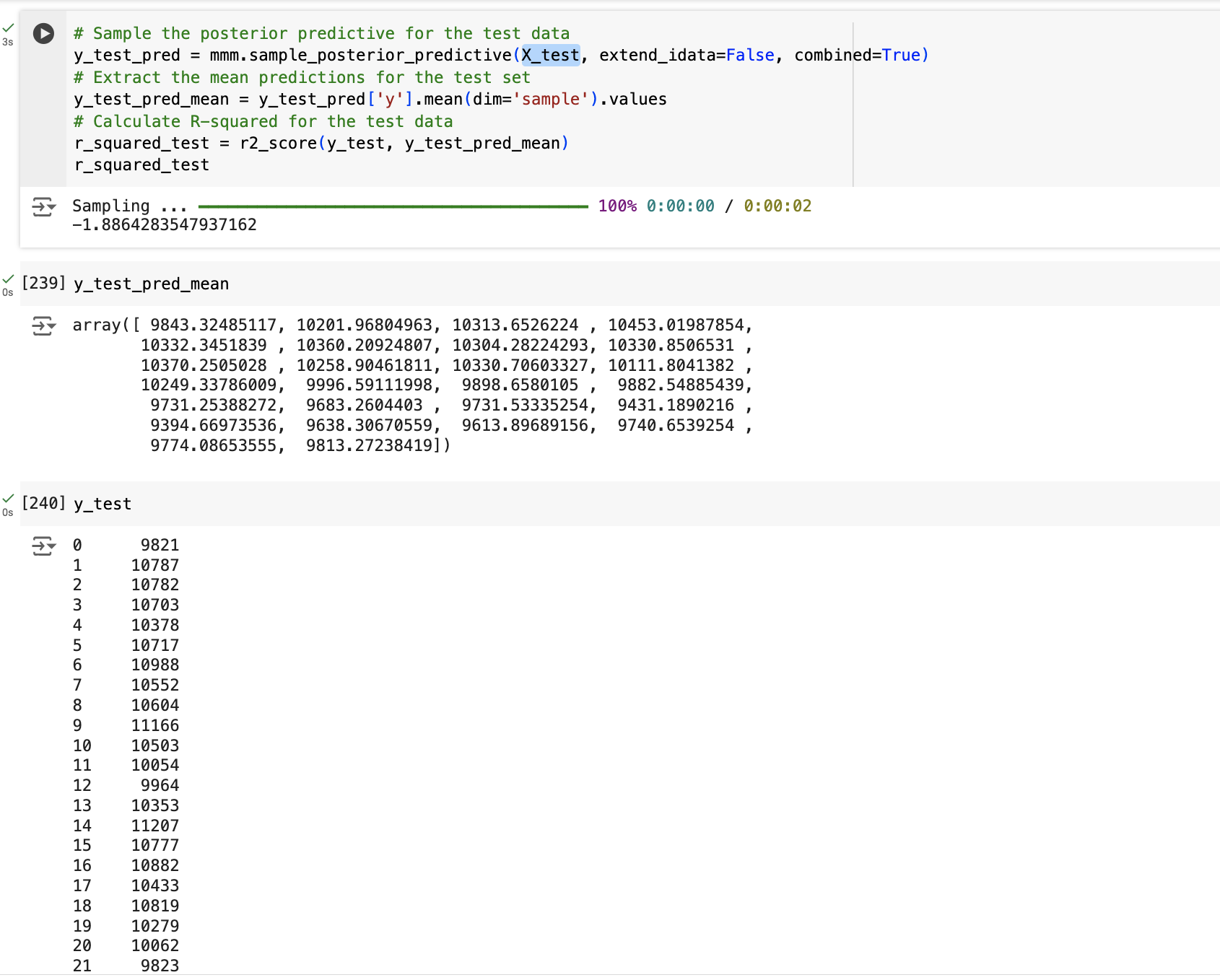
Thanks in advance!
Hi,
After I fit the model and try to get the R2 for my test data, I am getting negative R2. Can someone help me understand if I am calculating it correctly? The R2 for Train is 0.72.
Thanks in advance!
Assuming you are using sklearn’s r2_score function, the values can range from 1.0 to negative infinity:
Best possible score is 1.0 and it can be negative (because the model can be arbitrarily worse). In the general case when the true y is non-constant, a constant model that always predicts the average y disregarding the input features would get a
score of 0.0.
Thank for your response @cluhmann. Yes, I am using sklearn’s r2_score function. Does this mean that we cannot use R2 for model evaluation? If so, what would be the best metric to evaluate model strength?
Also, @cluhmann - How do you resolve this issue?
That function may be useful. There is no singular answer to the question “What is the correct metric to evaluate my model”? I might suggest checking out the notebooks on conducting posterior predictive checks.
Can we use sklearn R2 to compare the performance on out of sample dataset? Or is MAPE more reliable here to use?
You can use anything you’d like, but be aware that you should not take the mean of the posterior and compute a single statistic. You should compute the statistic for each posterior sample, then report the distribution over r2/mape/whatever
This gets very subtle and trips up a lot of new Bayesians trying to plug in the classical R^2 calculations. Here’s a nice overview from Gelman et al.
R-squared for Bayesian regression models. Andrew Gelman, Ben Goodrich, Jonah Gabry, Aki Vehtari. 2018. https://sites.stat.columbia.edu/gelman/research/unpublished/bayes_R2_v3.pdf
As warmup, the Wikipedia article on R^2 is nice:
You’re absolutely right of course. I believe arviz.r2_score does the computation based on the paper you linked. My post was more of a general tut-tutting about going through all the effort to sample a posterior via MCMC, only to reduce it to a point estimate to compute a metric of interest.
In general, metrics like MAPE/RMSE/etc are going to have some non-linearity, so Jensen’s Inequality rears its ugly head. What someone likely wants is the posterior mean out-of-sample whatever, but what he’s computing the the out-of-sample whatever of the posterior mean, which is not the same thing.
I’m with you on tut-tutting not doing proper Bayesian posterior predictive inference for quantities of interest.
It’s even more confusing when you need to estimate a log expected probability rather than an expected log probability. For the former, you have to be careful of precision and use the log-sum-exp trick. For the latter, it’s the issue you brought up about Jensen’s inequality. This is all pretty straightforward applications of a few common tricks once you get used to it, but I found it really really confusing to learn.