Application in social science: Outliers, priors, and negative binomial regression model

Dear all,

I am currently working on a research project where I would like to apply what I have learned in this course into practice. Sorry in advance that this post is quite long because (1) applying the knowledge and skills into real-world data has brought me a lot of questions, and (2) I would like to provide information that is as detailed as I can so that you can help with navigating the problems. Thank you so much for your guidance!!

List of questions:

  • Question 1: Interpretation based on correlation and scatterplot
  • Question 2 - Outliers
  • Questions 3.1 & 3.2 - All about priors

The context of the project:

  • Outcome variable: the number of green technology patents at time period t+1
  • Explanatory variable: the number of natural disasters at the time period t.
  • Unit of analysis: Indian states across different time periods.

I would like to know whether there is any relationship between these two variables in Indian states. Put differently, the research question is whether having a lot of natural disasters during this time period would make the Indian states more likely to produce more green technology patents in the next time period?

The data frame looks like this:

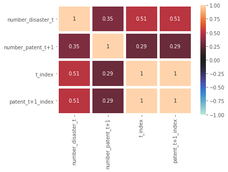
The correlation heat map looks like this:

image

The pairplot looks like this:

Question 1 - Interpretation based on correlation and scatterplot

Unlike the fish example that we have in the course, the scatterplot about the variables ‘number_disaster_t’ and ‘number_patent_t+1’ are not that linear. Instead, they are quite spread across the graph with no clear shapes. This might indicate that their correlation is not that strong and the relationship is not that linear. However, I have noticed that their correlation (shown in the correlation heat map) is 0.35. As a social scientist, I personally think that this is already very good because the correlation is above 0.25.

Thus, these pieces of information seem to be contradictory to me, and I am not sure how to interpret this. In addition, I am wondering whether I can still use a generalized linear regression to understand the relationship between these two variables?

Question 2 - Outliers

As green technology is somewhat new, there are not many patents in this field in the previous time periods (see the figure as the distribution of green technology patents by time period below).

In particular, if I zoom into the number of green technology patents that each state had, the variation is very big - some states had a lot of these patents (the most outstanding outlier had even around 30,000 patents in one period) while other states had very few of them.

Thus, my question here is whether I should remove those outliers shown in the following box plot?

Now questions about modelling:

I constructed a negative binomial regression model because (1) the number of patent is count data, and (2) the variance of the outcome variable is much larger than its mean (see the next figure):

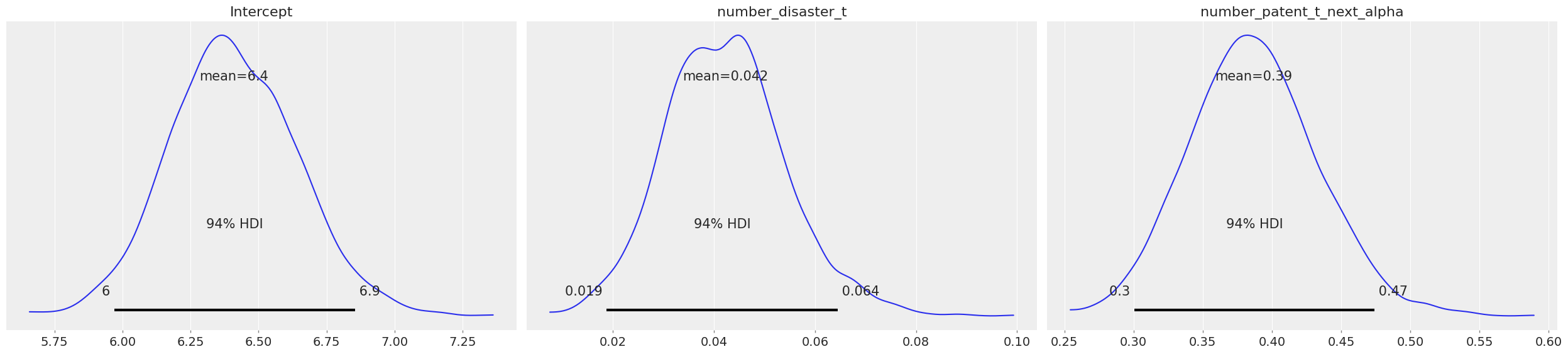
The first version of my Bayesian negative binomial regression model (with very small priors) is shown as below:

COORDS = {
    'slopes': ['number_disaster_t'], 
}

with pm.Model(coords=COORDS) as green_tech_without_control:
    # Data
    number_disaster_t = pm.ConstantData('number_disaster_t', 
                                         df.number_disaster_t.values,)

    # Prior
    intercept = pm.Normal('intercept', mu=0, sigma=1)
    β = pm.Normal('β', mu=0, sigma=1, dims=('slopes'))

    alpha = pm.Exponential('alpha', 0.5)

    # Linear regression
    mu = pm.math.exp(
        intercept
        + β[0] * number_disaster_t
    )

    # Likelihood, y_estimated
    pm.NegativeBinomial(
        'number_patent_t+1',
        mu=mu,
        alpha=alpha,
        observed=df['number_patent_t+1'].values,
    )

The outputs:

However, I encountered an error while trying to plot the prior predictive check, and is it caused by my misspecifying the model (i.e., wrong priors)?

The result of the posterior predictive check:

Question 3.1 - Priors

I chose the below priors just because they are from the example of how to build negative binomial regression in PyMC. To be honest, I am not quite sure about what those priors that I set really mean:

# Prior
    intercept = pm.Normal('intercept', mu=0, sigma=1)
    β = pm.Normal('β', mu=0, sigma=1, dims=('slopes'))

    alpha = pm.Exponential('alpha', 0.5)

Based on my intuition, intercept indicate the mean value of my outcome variable (the number of green patents in time t+1) when the explanatory variable (the number of natural disasters in time t) is 0, what I know is that it has to be positive. As it is count data, I am wondering why here we are using a normal distribution, instead of a distribution for count data?

If it is going to follow Poisson or Negative binomial distribution, is it going to be very duplicated like how I defined likelihood here (see the line of code below)?

# Likelihood, y_estimated
    pm.NegativeBinomial(
        'number_patent_t+1',
        mu=mu,
        alpha=alpha,
        observed=df['number_patent_t+1'].values,
    )

Question 3.2 - Priors

I wanted to change the priors of intercept and slope to better fit my own expectations, but the code below had an issue while doing MCMC sampling.

The code is as below:

COORDS = {
    'slopes': ['number_disaster_t'], 
}

with pm.Model(coords=COORDS) as green_tech_without_control:
    # Data
    number_disaster_t = pm.ConstantData('number_disaster_t', 
                                         df.number_disaster_t.values,)

    # Prior
    intercept = pm.Normal('intercept', mu=1, sigma=10) # I even tried sigma=1000 but MCMC sampling also failed. 
    β = pm.Normal('β', mu=0, sigma=10, dims=('slopes'))

    alpha = pm.Exponential('alpha', 0.5)

    # Linear regression
    mu = pm.math.exp(
        intercept
        + β[0] * number_disaster_t
    )

    # Likelihood, y_estimated
    pm.NegativeBinomial(
        'number_patent_t+1',
        mu=mu,
        alpha=alpha,
        observed=df['number_patent_t+1'].values,
    )

Error:


The full information about the hints provided by the error display:

  • HINT: Re-running with most Aesara optimizations disabled could provide a back-trace showing when this node was created. This can be done by setting the Aesara flag ‘optimizer=fast_compile’. If that does not work, Aesara optimizations can be disabled with ‘optimizer=None’.
  • HINT: Use the Aesara flag exception_verbosity=high for a debug print-out and storage map footprint of this Apply node.

May I know how to solve this problem?

Many thanks again for your support :smiling_face_with_three_hearts:

2 Likes

Thank you Yuqi for this detailed post which contains all the relevant details, including both data and a model graph!

For context for others when the course is mentioned it’s the Intuitive Bayes Introductory Course. I asked this question be moved here so answers can be captured for wider benefit.

Let me try and go through each question in turn

Question 1

The assumption of linear correlation is a modeling decision. You mention one measure which of linerarity pearson’s correlation coefficient which can help inform things, but as you noticed things can be confusing when summary metrics are compared with visualizations.

The classic example of this is Anscombes Quartet

For your problem what I’d suggest is thinking through a couple of different models. If we assume the relationship is not linear, what kind of relationship would we expect? The beauty of Bayesian models, especially in PyMC, is that you can specify whatever type of relationship you want in the code. This flexibility is a big part of why I use PPLs

Other Questions

For questions 2, 3.1, and 3.2 I’ll come back with longer answers later today (ran of time now) Quickly for question 3 I suggest taking a look at the preliz library and using prior predictive functionality. You’re having some other issues, I’ll come back and give a better answer later today

Use PyMC v5

Also in regards to the libraries, I suggest upgrading to the latest version of PyMC, which is now on v5, which uses pytensor, I know in the course we use PyMC v4. The overall PyMC team moves quickly though and we’re always making changes to make the PPL better. Great for users, bad for course creators who have to pick one version when they make a course :sweat:

2 Likes

Thanks a lot @RavinKumar for your prompt reply with many helpful insights!!

Regarding your answer to Question 1, I hope that you don’t mind if I am asking two more questions here:

I have taken the scatterplot about the outcome variable and explanatory variable out of the pair plot so that the information is clearer and more targeted:

I noticed that there are so many observations located in the bottom-left corner, thus I thought about zooming into it and see whether there is a clear trend:

However, unfortunately there is still no clear shape.

Question 1.1 - Non-linear models

Coming from a background in social sciences, I have to say that I have been used to fit almost everything into (generalized) linear regression models without critically thinking about why I should do that. The course and the chance to discuss with you in this way have helped me a lot to understand statistics in a much deeper way and build a systematic workflow.

As I am not very familiar with non-linear regression models, could you please give more detailed suggestions regarding which directions I could go in this application? I am also enrolled in the course about Gaussian Processes, and I am wondering whether I can build a Gaussian process regression model?

Moreover, one thing that I am concerned about is that the scatterplot doesn’t indicate strongly that it has a curved shape, too. Thus I am wondering which type of non-linear regression model would be the best fit here.

Question 1.2 - Data transformation

In the introductory course, you use the fish example to explain that, if we would like to fit a linear regression model, then it is necessary to transform the variables so that the relationship is linear. In that case, we logged the variables to do so.

In this Indian states’ example, since we cannot see a curved or linear shape here, I am wondering whether we can still think about doing data transformation? Or put differently to make it more generalizable, in which occasions should we think about transforming our data?

Sorry for such a long post with questions again :exploding_head: Your efforts and support are really appreciated :heart:

1 Like

No need to apologize for the questions! It’s all part of the learning process.

Looking over all the questions, they all seem to point to the same latent idea which is “How do i construct and model and how do I feel comfortable with my choices?”

That question is basically the Bayesian workflow in which you iterate through these steps to get to a model you can justify

https://bayesiancomputationbook.com/markdown/chp_09.html#fig-bayesianworkflow

For your problem specifically a linear model seems like a good start. In the basic model it presupposes that the same effect is present for all time periods and all states.

The questions I have off the bat are

  1. Is the relationship indeed linear? As you mentioned for the fish regression a transformation was needed for a better linear fit. The same idea is explained here as well
    4. Extending Linear Models — Bayesian Modeling and Computation in Python… You’ve already created a plot showing there isn’t much of a relationship at least in EDA, but maybe its linear enough to be useful? I’m not sure how strong your conclusions need to be
  2. For the question about outliers, t’d ask do you think it a true outlier unrepresentative of the data generating process? If so then removing it sounds fine to me. The other strategy in bayesian modeling is leaving it in but using a prior that heavily regularizes the posterior, though this should come with strong justification
  3. I don’t think Gaussian processes should be a go to modeling technique here. It doesn’t look like there has been basic regressions performed where you control for the state. It may be that hierarchical either on state or the time period dimension may yield better results. In the intro course @twiecki does a great job explaining the intuition, and this notebook shows the classic radon example
    GLM: Hierarchical Linear Regression — PyMC3 3.11.4 documentation

Lastly if you’re doing a lot of regressions consider using Bambi. It’s a really great tool and for linear models especially can speed up your iteration.

This is all quite a bit of info so it may take a while to parse through. Hope this gives you a couple good directions to consider.

2 Likes

Hi Ravin @RavinKumar, many thanks for your very helpful guidance! I have updated my PyMC to the latest version and now using Bambi to run my negative binomial regression models. I would like to ask you two questions this time:

List of questions

  • Question 1: Sampling error

With Bambi, I could run the simplest model (outcome variable ~ explanatory variable), but not able to run the model when I added two control variables (outcome variable ~ explanatory variable + control variable 1 + control variable 2).

  • Question 2: Missing values

The details will be elaborated below:

Question 1: Sampling error

Model 1

model = bmb.Model('number_patent_t_next ~ number_disaster_t', 
                  df, 
                  family="negativebinomial")

fitted_results = model.fit()

Results:

Model 2

Apart from the outcome and explanatory variables, I added two control variables for each state during a particular time period, which are the median GDP and population of the state during the particular time period. Thus, the overall dataframe would look like this:

model = bmb.Model('number_patent_t_next ~ number_disaster_t + median_gdp_t + population_t', 
                  df, 
                  family="negativebinomial")

fitted_results = model.fit()
---------------------------------------------------------------------------
SamplingError                             Traceback (most recent call last)
Cell In[17], line 5
      1 model = bmb.Model('number_patent_t_next ~ number_disaster_t + median_gdp_t + population_t', 
      2                   df, 
      3                   family="negativebinomial")
----> 5 fitted_results = model.fit()

File /opt/anaconda3/envs/dphil/lib/python3.10/site-packages/bambi/models.py:325, in Model.fit(self, draws, tune, discard_tuned_samples, omit_offsets, include_mean, inference_method, init, n_init, chains, cores, random_seed, **kwargs)
    318     response = self.components[self.response_name]
    319     _log.info(
    320         "Modeling the probability that %s==%s",
    321         response.response_term.name,
    322         str(response.response_term.success),
    323     )
--> 325 return self.backend.run(
    326     draws=draws,
    327     tune=tune,
    328     discard_tuned_samples=discard_tuned_samples,
    329     omit_offsets=omit_offsets,
    330     include_mean=include_mean,
    331     inference_method=inference_method,
    332     init=init,
    333     n_init=n_init,
    334     chains=chains,
...
{'number_patent_t_next_alpha_log__': array(-0.03759918), 'Intercept': array(0.18543183), 'number_disaster_t': array(0.57930111), 'median_gdp_t': array(-0.92960239), 'population_t': array(-0.3263707)}

Logp initial evaluation results:
{'number_patent_t_next_alpha': -1.15, 'Intercept': -2.48, 'number_disaster_t': -5.95, 'median_gdp_t': -513852195.53, 'population_t': -11084021.48, 'number_patent_t_next': -inf}
You can call `model.debug()` for more details.
model.debug()
---------------------------------------------------------------------------
AttributeError                            Traceback (most recent call last)
Cell In[9], line 1
----> 1 model.debug()

AttributeError: 'Model' object has no attribute 'debug'

I find that this part is a bit weird:

Logp initial evaluation results:
{'number_patent_t_next_alpha': -1.15, 'Intercept': -2.48, 'number_disaster_t': -5.95, 'median_gdp_t': -513852195.53, 'population_t': -11084021.48, 'number_patent_t_next': -inf}
You can call `model.debug()` for more details.

Here, all the values after the Logp initial evaluation are negative. As a newbie, unfortunately, I haven’t gained a deep understanding about how the mechanisms work under the hood. Could you please explain a bit so that I can better understand this? And any suggestions regarding what I should do to solve this sampling error issue?

Question 2: Missing values

I am not sure whether the sampling error issue is related to missing values in the dataframe (screenshot below). I tried to replace null values by 0; however, it doesn’t really help and the sampling error issue still exists. As to the missing values issue, I have the following questions:

2.1 How are regression models influenced by missing values?
2.2 How should we deal with missing values? And in this case?

Thank you so much and have a lovely day ahead!
Yuqi

For the model.debug() issue there might be a bug in bambi, Can you create a minimal example and post it here?

Basically the sampler is trying to find a place to start sampling but it’s unable to. This is either an issue with the model, the priors, or the data but I can’t tell which without the full notebook.

One way to check if what you think is happening is indeed happening is with a parameter recovery study. In scipy/numpy create a linear function that outputs data like the one youre studying, and just put in arbitrary parameters. Then use bambi and see if you can recover those parameters.

For missing values, that is going to depend on your domain and your analysis, more than on the model. putting 0 might mess up your regression. Maybe the prevalence of missing values is so slow you can drop those values and do complete case analysis, but the assumption there of course is that the missing. values aren’t correlated with some factor of interest.

So in summary

  1. Try doing parameter recovery study first, that’ll ensure that the model is working correctly
  2. Think hard about what missing data means and make a judgement call on what to do, dont let the sampler drive your analysis