Hey Everyone,
I am working on a source separation model. The model is as follows:
Y = E + D*log_{10}(AS) + \epsilon
E ~ Normal(0.1, \sigma_e*E_{temp})
E_{temp} ~ Normal(0,1)
D ~ Normal(0.055, \sigma_d*D_{temp})
D_{temp} ~ Normal(0,1)
A ~ Uniform(0,1)
S ~ HalfNormal(\sigma=1)
\epsilon ~ Normal(0, 1)
Some more notes on the model:
E is a matrix of shape (num_electrodes, num_samples) where each row is the same. For e.g E = [[1,1,1,1,1],
[2,2,2,2,2],
[3,3,3,3,3]]
D is a diagonal matrix. of shape (num_electrodes, num_sources)
A is a matrix of shape (num_electrodes, num_sources) and its diagonal elements are 1
S is a matrix of shape (num_sources, num_samples)
You will see in the code that I do several matrix operations to transform the random variables into this form.
Here is the code:
import numpy as np
import matplotlib.pyplot as plt
from sklearn.preprocessing import StandardScaler, MinMaxScaler
import pymc3 as pm
import matplotlib.pyplot as plt
import arviz as az
import theano as tt
%matplotlib inline

########## generate data ######
num_samples = 50
num_electrodes = 3
num_sources = 3
AA = np.array([[1, 0.16, 0.40], [0.25, 1, 0.19], [0.40, 0.13, 1]])
d = [[0.059], [0.050], [0.055]]
e = [[0.095], [0.105], [0.110]]

s1 = (2 + np.sin(np.linspace(0,10, num_samples)))*0.2
s2 = (2 + np.sin(np.linspace(5,8, num_samples)))*0.2
s3 = (2 + np.sin(np.linspace(2,4, num_samples)))*0.2

S_comb = np.power([s1,s2,s3],1)
plt.figure(figsize=(10,5))
a= plt.plot(S_comb.T)
plt.legend(['s1','s2','s3'])

s_mean = 0
s_sigma = 0.5
noise_sigma = 0.0005
EE = np.matmul(e, np.ones((1, num_samples)))
DD = np.diag(np.array(d).T[0])
SS = S_comb
Y = EE + np.matmul(DD , np.log10(np.matmul(AA, SS)))
Y_obs = Y + np.random.normal(loc=0, scale=noise_sigma, size=Y.shape)

print(EE.shape)
print(DD.shape)
print(Y.shape)
plt.figure(figsize=(12,6))
plt.plot(Y_obs.T, marker='o')

##### Model ####
samples = 2000
tune = 1000
with pm.Model() as model:
  sigma_E = 0.02*pm.HalfNormal('sigma_E', sigma=1)
  sigma_D = 0.02*pm.HalfNormal('sigma_D', sigma=1)

  temp_E1 = pm.Normal('temp_E1', mu=0, sigma=1, shape=(1,num_electrodes))
  E1 =  pm.Deterministic('E1', 0.1 + sigma_E*temp_E1)
  E = pm.Deterministic('E', pm.math.dot(E1.T, np.ones((1,num_samples))))

  diag = tt.shared(np.diag(np.ones(num_electrodes)))
  temp_D1 = pm.Normal('temp_D1', sigma=1, shape=(1,num_electrodes))
  m = pm.math.dot(temp_D1.T, np.ones((1,num_electrodes)))
  D1 = diag*m
  D = pm.Deterministic('D', 0.055*diag + sigma_D*D1)

  temp_A = pm.Uniform('temp_A', lower=0, upper=1, shape=(num_electrodes,num_sources))
  a1 = np.ones((num_electrodes,num_sources))
  np.fill_diagonal(a1, 0)
  a2 = np.zeros((num_electrodes,num_sources))
  np.fill_diagonal(a2, 1)
  diag1 = tt.shared(a1)
  diag2 = tt.shared(a2)
  temp_A1 = pm.Deterministic('temp_A1', temp_A*a1)
  A = pm.Deterministic('A', temp_A1 + a2)

  S = pm.HalfNormal('S', sigma=1, shape=(num_sources,num_samples))

  sigma_temp= pm.HalfNormal('sigma_temp', sigma=1)
  #sigma = pm.Deterministic('sigma', sigma_temp/scaler_std)

  y_mean = E + pm.math.dot(D, np.log10(pm.math.dot(A, S)))
  #y_mean = (E + pm.math.dot(D , np.log10(pm.math.dot(A, S))) - scaler_mean)/scaler_std
  obs = pm.Normal('obs', mu=y_mean, sigma=sigma_temp, observed=Y_obs)
  #obs = pm.StudentT('obs', nu=2, mu=y_mean, sigma=sigma, observed=scaled_Y.T)
  #start = pm.find_MAP()
  #prior_checks = pm.sample_prior_predictive(samples=50)
  trace0 = pm.sample(samples, tune=tune, chains=2, cores=1, target_accept=0.9)
The trace is as follows:
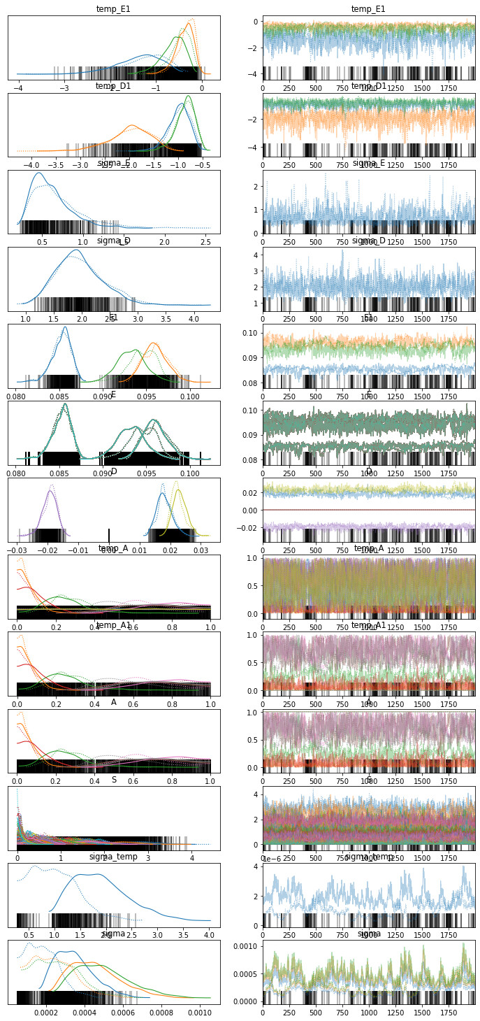
I have tried non centered parametrization and also bumped up the target_accept but with no avail. Any insights into why this is happening is appreciated.