Clinical Trial data - request help on variable number of comparisons per trial

I have data for 36 studies with binomial data for 7 medical treatments. For each trial I have the number of patients, and the number who had an event of interest. Most of the studies have 2 arms, but the first study has 3 arms. I am trying to write code that treats the data the same way as what is in Technical support document 2 on the NICE website, and what is in the book “Network Meta-Analysis for Decision-Making”

I wrote code for two arms, but now I want to have it handle the one case with 3 arms. Latter I will have to add a bias correction for 3 arms trials, but for now I just want to add the single case with 3 arms.

This is not a missing data problem. I would appreciate any help or suggestions on how to handle the 3rd arm.

Hopefully the code below is better formatted than on my first try.

import arviz as az
import matplotlib.pyplot as plt
import pandas as pd
import numpy as np
import pymc as pm
import pytensor.tensor as pt
import pytensor 
%matplotlib inline


mport pandas as pd
import io
data_string="""studyID,na,t1,t2,t3,r1,n1,r2,n2,r3,n3,study
1,3,1,3,4,1472,20251,652,10396,723,10374,GUSTO-1 1993
2,2,1,2,,3,65,3,64,,,ECSG 1985
3,2,1,2,,12,159,7,157,,,TIMI-1 1987
4,2,1,2,,7,85,4,86,,,PAIMS 1989
5,2,1,2,,10,135,5,135,,,White 1989
6,2,1,2,,887,10396,929,10372,,,GISSI-2 1990
7,2,1,2,,5,63,2,59,,,Cherng 1992
8,2,1,2,,1455,13780,1418,13746,,,ISIS-3 1992
9,2,1,2,,9,130,6,123,,,CI 1993
10,2,1,4,,4,107,6,109,,,KAMIT 1991
11,2,1,5,,285,3004,270,3006,,,INJECT 1995
12,2,1,7,,11,149,2,152,,,Zijlstra 1993
13,2,1,7,,1,50,3,50,,,Riberio 1993
14,2,1,7,,8,58,5,54,,,Grinfeld 1996
15,2,1,7,,1,53,1,47,,,Zijlstra 1997
16,2,1,7,,4,45,0,42,,,Akhras 1997
17,2,1,7,,14,99,7,101,,,Widimsky 2000
18,2,1,7,,9,41,3,46,,,DeBoer 2002
19,2,1,7,,42,421,29,429,,,Widimsky 2002
20,2,2,7,,2,44,3,46,,,DeWood 1990
21,2,2,7,,13,200,5,195,,,Grines 1993
22,2,2,7,,2,56,2,47,,,Gibbons 1993
23,2,3,5,,13,155,7,169,,,RAPID-2 1996
24,2,3,5,,356,4921,757,10138,,,GUSTO-3 1997
25,2,3,6,,522,8488,523,8461,,,ASSENT-2 1999
26,2,3,7,,3,55,1,55,,,Ribichini 1996
27,2,3,7,,10,94,3,95,,,Garcia 1997
28,2,3,7,,40,573,32,565,,,GUSTO-2 1997
29,2,3,7,,5,75,5,75,,,Vermeer 1999
30,2,3,7,,5,69,3,71,,,Schomig 2000
31,2,3,7,,2,61,3,62,,,LeMay 2001
32,2,3,7,,19,419,20,421,,,Bonnefoy 2002
33,2,3,7,,59,782,52,790,,,Andersen 2002
34,2,3,7,,5,81,2,81,,,Kastrati 2002
35,2,3,7,,16,226,12,225,,,Aversano 2002
36,2,3,7,,8,66,6,71,,,Grines 2002"""
data=pd.read_csv(io.StringIO(data_string),sep=",")

trials=data[["n1","n2"]]
events=data[["r1","r2"]]
trt=data[["t1","t2"]].to_numpy()-1
N=len(trials)
studies=data["study"]
treatments=["SK","t-PA","at-PA","SK+t-PA","r-PA","TNK","PTCA"]
coords = {"studies": studies, "treatments":treatments}
reference=np.array([0,1,1,1,1,1,1])

with pm.Model(coords=coords) as femodel:
    r=pm.MutableData('r',events)
    n=pm.MutableData('n',trials)
    t=pm.MutableData('t',trt)    
    d_=pm.Normal("d_",mu=0,sigma=100,dims="treatments")
    d=pm.Deterministic("d",d_*reference,dims="treatments")
    mu=pm.Normal("mu",mu=0,sigma=100,dims="studies",shape=(N,1))
    dm=pm.Deterministic("dm",d[t])
    linpred=pm.Deterministic("linpred",mu+dm)
    p=pm.Deterministic("p",pm.invlogit(linpred))
    y=pm.Binomial("y",n=n,p=p,observed=r)

    fedata=pm.sample(10000,tune=5000, nuts_sampler="nutpie")

pm.model_to_graphviz(femodel2)

pm.model_to_graphviz(femodel2)
You can style your code using three single ticks ``` before and after whole of the code. Can you upload the data as a csv file and link here? There are 12 columns in the header and first row but 9 in others and they seem to have shifted (because of different number of arms probably).

That is ok, from the text file I was able to get the excel and run the code. There are some things which does not make sense to start with:

You create a variable “d_” with seven elements. Two things I don’t understand is later you transform it via

d=pm.Deterministic("d",d_*reference,dims="treatments")

which only has the effect of making d[0] 0 and keeping other d the same. Due to the structure of your model later on, d_[0] therefore does not contribute to anything. On top of this you later on do:

dm=pm.Deterministic("dm",d[t])

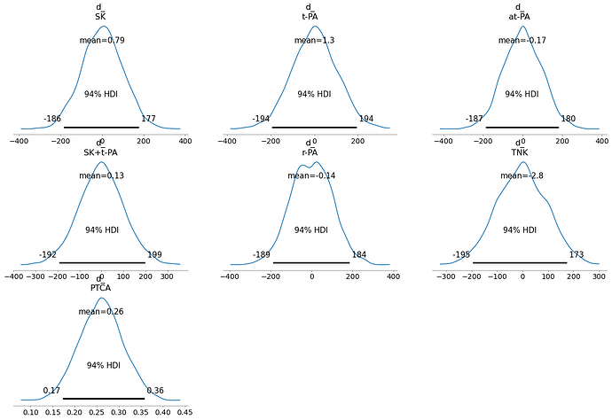
and you go on to use. However t is an indexer that simply picks the last and first element of d and tiles it, therefore anything other than the first and last element gets discarded basically (as they are not used elsewhere). With the fact that you set d_ to 0 before, basically only thing that matters for your model is d_[-1]. And indeed this is why the posterior plots for d_ look like

As you can see anything other than d_[-1] is exactly the same as your prior, very large normal distributions. If you only care about the last element, you probably don’t need to create others? For others interested, the code I am using is as follows:

import arviz as az
import matplotlib.pyplot as plt
import pandas as pd
import numpy as np
import pymc as pm
import pytensor.tensor as pt
import pytensor 

import pandas as pd
import io
blocker_string="""
study,na,r1,r2,n1,n2,t1,t2
1,2,3,3,39,38,0,1
2,2,14,7,116,114,0,1
3,2,11,5,93,69,0,1
4,2,127,102,1520,1533,0,1
5,2,27,28,365,355,0,1
6,2,6,4,52,59,0,1
7,2,152,98,939,945,0,1
8,2,48,60,471,632,0,1
9,2,37,25,282,278,0,1
10,2,188,138,1921,1916,0,1
11,2,52,64,583,873,0,1
12,2,47,45,266,263,0,1
13,2,16,9,293,291,0,1
14,2,45,57,883,858,0,1
15,2,31,25,147,154,0,1
16,2,38,33,213,207,0,1
17,2,12,28,122,251,0,1
18,2,6,8,154,151,0,1
19,2,3,6,134,174,0,1
20,2,40,32,218,209,0,1
21,2,43,27,364,391,0,1
22,2,39,22,674,680,0,1"""
data=pd.read_csv(io.StringIO(blocker_string),sep=",")

trials=data[["n1","n2"]]
events=data[["r1","r2"]]
trt=data[["t1","t2"]].to_numpy()-1
N=len(trials)
studies=data["study"]
treatments=["SK","t-PA","at-PA","SK+t-PA","r-PA","TNK","PTCA"]
coords = {"studies": studies, "treatments":treatments}
reference=np.array([0,1,1,1,1,1,1])

with pm.Model(coords=coords) as femodel:
    r=pm.MutableData('r',events)
    n=pm.MutableData('n',trials)
    t=pm.MutableData('t',trt)    
    
    d_=pm.Normal("d_",mu=0,sigma=100,dims="treatments")
    d=pm.Deterministic("d",d_*reference,dims="treatments")
    
    mu=pm.Normal("mu",mu=0,sigma=100,dims="studies",shape=(N,1))
    dm=pm.Deterministic("dm",d[t])
    
    
    linpred=pm.Deterministic("linpred",mu+dm)
    p=pm.Deterministic("p",pm.invlogit(linpred))
    y=pm.Binomial("y",n=n,p=p,observed=r)

    fedata=pm.sample(1000,tune=500)

pm.model_to_graphviz(femodel)

I’m trying to replicate the winbugs code below:

For the reference group they set it to d[1]<-0. I’m trying to get the same thing, but was having trouble putting a 0 and 6 Normal random variables in the same vector.

I don’t like that I’m creating a normal random variable and then ignoring it. This was going to be a follow-up question.

# Binomial likelihood, logit link
# Fixed effect model 
model{                          # *** PROGRAM STARTS
for(i in 1:ns){                 # LOOP THROUGH STUDIES
    mu[i] ~ dnorm(0,.0001)      # vague priors for all trial baselines
    for (k in 1:na[i])  {       # LOOP THROUGH ARMS
        r[i,k] ~ dbin(p[i,k],n[i,k])    # binomial likelihood
        logit(p[i,k]) <- mu[i] + d[t[i,k]] - d[t[i,1]]
      }
     }   
d[1]<-0    # treatment effect is zero for reference treatment
# vague priors for treatment effects
for (k in 2:nt){  d[k] ~ dnorm(0,.0001) }
}                                                     # *** PROGRAM ENDS

Hmm I am not super familiar with winbugs but I think I get roughly what is going on here. What does t[i,k] look like in their case? In the first code you have supplied they are different files but in the text file you have attached it is always 0 and 1 which might be a mistake?

blocker_string="""
study,na,r1,r2,n1,n2,t1,t2
1,2,3,3,39,38,0,1
2,2,14,7,116,114,0,1
3,2,11,5,93,69,0,1
4,2,127,102,1520,1533,0,1
5,2,27,28,365,355,0,1
6,2,6,4,52,59,0,1
7,2,152,98,939,945,0,1
8,2,48,60,471,632,0,1
9,2,37,25,282,278,0,1
10,2,188,138,1921,1916,0,1
11,2,52,64,583,873,0,1
12,2,47,45,266,263,0,1
13,2,16,9,293,291,0,1
14,2,45,57,883,858,0,1
15,2,31,25,147,154,0,1
16,2,38,33,213,207,0,1
17,2,12,28,122,251,0,1
18,2,6,8,154,151,0,1
19,2,3,6,134,174,0,1
20,2,40,32,218,209,0,1
21,2,43,27,364,391,0,1
22,2,39,22,674,680,0,1"""

This is what the winbugs code looks like (data with a third arm). In the software you select the data and hit a load button. Notice that the first row of data is the only row with a third arm.

na[]	t[,1]	t[,2]	t[,3]	r[,1]	n[,1]	r[,2]	n[,2]	r[,3]	n[,3]	#	ID	year
3	1	3	4	1472	20251	652	10396	723	10374	#	GUSTO-1	1993
2	1	2	NA	3	65	3	64	NA	NA	#	ECSG	1985
2	1	2	NA	12	159	7	157	NA	NA	#	TIMI-1	1987
2	1	2	NA	7	85	4	86	NA	NA	#	PAIMS	1989
2	1	2	NA	10	135	5	135	NA	NA	#	White	1989
2	1	2	NA	887	10396	929	10372	NA	NA	#	GISSI-2	1990
2	1	2	NA	5	63	2	59	NA	NA	#	Cherng	1992
2	1	2	NA	1455	13780	1418	13746	NA	NA	#	ISIS-3	1992
2	1	2	NA	9	130	6	123	NA	NA	#	CI	1993
2	1	4	NA	4	107	6	109	NA	NA	#	KAMIT	1991
2	1	5	NA	285	3004	270	3006	NA	NA	#	INJECT	1995
2	1	7	NA	11	149	2	152	NA	NA	#	Zijlstra	1993
2	1	7	NA	1	50	3	50	NA	NA	#	Riberio	1993
2	1	7	NA	8	58	5	54	NA	NA	#	Grinfeld	1996
2	1	7	NA	1	53	1	47	NA	NA	#	Zijlstra	1997
2	1	7	NA	4	45	0	42	NA	NA	#	Akhras	1997
2	1	7	NA	14	99	7	101	NA	NA	#	Widimsky	2000
2	1	7	NA	9	41	3	46	NA	NA	#	DeBoer	2002
2	1	7	NA	42	421	29	429	NA	NA	#	Widimsky	2002
2	2	7	NA	2	44	3	46	NA	NA	#	DeWood	1990
2	2	7	NA	13	200	5	195	NA	NA	#	Grines	1993
2	2	7	NA	2	56	2	47	NA	NA	#	Gibbons	1993
2	3	5	NA	13	155	7	169	NA	NA	#	RAPID-2	1996
2	3	5	NA	356	4921	757	10138	NA	NA	#	GUSTO-3	1997
2	3	6	NA	522	8488	523	8461	NA	NA	#	ASSENT-2	1999
2	3	7	NA	3	55	1	55	NA	NA	#	Ribichini	1996
2	3	7	NA	10	94	3	95	NA	NA	#	Garcia	1997
2	3	7	NA	40	573	32	565	NA	NA	#	GUSTO-2	1997
2	3	7	NA	5	75	5	75	NA	NA	#	Vermeer	1999
2	3	7	NA	5	69	3	71	NA	NA	#	Schomig	2000
2	3	7	NA	2	61	3	62	NA	NA	#	LeMay	2001
2	3	7	NA	19	419	20	421	NA	NA	#	Bonnefoy	2002
2	3	7	NA	59	782	52	790	NA	NA	#	Andersen	2002
2	3	7	NA	5	81	2	81	NA	NA	#	Kastrati	2002
2	3	7	NA	16	226	12	225	NA	NA	#	Aversano	2002
2	3	7	NA	8	66	6	71	NA	NA	#	Grines	2002
END

Ok we are getting somewhere. For anyone interested code is below. I only had to make some slight changes which I think made the models the same:

dm=pm.Deterministic("dm",d[trt]-d[trt[:,0:1]])

This effectively vectorizes the loop that they were doing, Other parts vectorize automatically by broadcasting so no change was necessary. The posteriors that I now get are well defined for every study since they get all used

And how do you want to generalize this?


import arviz as az
import matplotlib.pyplot as plt
import pandas as pd
import numpy as np
import pymc as pm
import pytensor.tensor as pt
import pytensor


data=pd.read_csv("data.csv")

trials=data[["n1","n2"]]
events=data[["r1","r2"]]
trt=data[["t1","t2"]].to_numpy()-1
N=len(trials)
studies=data["study"]
treatments=["SK","t-PA","at-PA","SK+t-PA","r-PA","TNK","PTCA"]
coords = {"studies": studies, "treatments":treatments}
reference=np.array([0,1,1,1,1,1,1])

with pm.Model(coords=coords) as femodel:
    r=pm.MutableData('r',events)
    n=pm.MutableData('n',trials)

    d_=pm.Normal("d_",mu=0,sigma=100,dims="treatments")
    d=pm.Deterministic("d",d_*reference,dims="treatments")

    mu=pm.Normal("mu",mu=0,sigma=100,dims="studies",shape=(N,1))
    dm=pm.Deterministic("dm",d[trt]-d[trt[:,0:1]])

    linpred=pm.Deterministic("linpred",mu+dm)
    p=pm.Deterministic("p",pm.invlogit(linpred))
    y=pm.Binomial("y",n=n,p=p,observed=r)

    fedata=pm.sample(1000,tune=500)

az.plot_posterior(fedata)

data.csv (1.6 KB)

I’m going to try your code tomorrow morning. In the code I’m only reading the first two arms, my next step is to read all three arms, e.g. trials=data[[“n1”,“n2”,“n3”]] and deal with the fact that in most cases n3 has Nans

By the way, in this sort of problem performance is nice, but not so important. I’m working on aggregate data reported mostly in academic journals. So I will always be using small datasets. The focus is to, knock on wood, being correct in the analysis. I don’t think the source I’m trying to replicate is the last word, but is provided by regulators in the UK, so I would like to be able to do what they did before suggesting any changes.

Also, in this problem we are mostly interested in the differences between treatments. In the model the differences are a fixed effect. Each trial has it’s own mean to try to pick differences between clinical trials or studies (trials). In each individual study or trail, the patients are randomized, so they should have similar characteristics. However, when you compare study 1 with study 2, they would have had different rules for randomization and drawn from a pool of patients that are different. Hopefully, not too different.

If you want to track differences between different studies, you should not compare the posterior plots directly. You should keep track of it via something like

dif_mu = pm.Deterministic("dif_mu", mu - mu.T)

Here dif_mu[i,j] will give you the difference between mean of study i and j. Don’t mind the warnings about scalar divide, they happen because mu[i,i] - mu[i,i] is always zero.

The difference in means are not the focus. There are 36 studies and each will have a different mean. The study mean is used in each arm of the study. We are really interested in the 7 treatments and in comparing them with each other.

Another version of the model that is labeled a “random effects” has separate treatment effects for each treatment by study. I have coded this, and it’s a little more challenging to get the model to converge, but it did converge, and the mixing looks good, however, it seems that the sampler gets stuck in certain places for a not huge but not insignificant number of samples. I got this from looking at the plot along the axis below the distribution (you get 36 means, and 36 random treatment effects).

So basically the d-vector is the ball ball game and the other parameters are considered
nuisance parameter. Also, I might calculate things like odd ratios and some other measures either in the model or with the samples. It’s probably easier to have them in the model since they are named and tracked and ready without any additional data wrangling.

Thank you for taking the time to look at the model.

I think I will explore expanding the “na” column with the following code:

na=pd.DataFrame(np.array([[i,j-1,k+1] for i,j in enumerate(data[‘na’]) for k in np.arange(j-1)]))

In this case it extends the na’s from 36 to 37 rows. I hope that I can then feed it to the scan function as a sequence, along with other non sequenced variables to build the structures with variables in the right positions that I need.

I’m not sure how to code it or what the unknow unknows are going to be.

I want to develop along the lines of the code below:

import pytensor 
import pytensor.tensor as pt

na=pd.DataFrame(np.array([[i,j-1,k+1] for i,j in enumerate(data['na']) for k in np.arange(j-1)]))

with pm.Model() as model:
    #study_arms=pm.Deterministic("study_arms",na)
    study_arms=pm.MutableData('study_arms',na)
    
    def pairs(a):
        b=a[:2]
        return b

    outputs,_=pytensor.scan(fn=pairs,sequences=study_arms)
    foo=pm.Deterministic("foo",outputs)

    pm.model_to_graphviz(model)