Converting Model from Stan

I have a change point model in Stan

data {
  int<lower=1> N;
  vector[N] x;
  vector[N] y;
}

parameters {
  real tau;
  real mu1;
  real mu2;
  real gamma1;
  real gamma2;

  real<lower=0> sigma1;
  real<lower=0> sigma2;
}

model {
  real mu;
  real gamma;
  real sigma;

  mu1 ~ normal(0, 10);
  mu2 ~ normal(0, 10);
  gamma1 ~ normal(0, 10);
  gamma2 ~ normal(0, 10);
  sigma1 ~ normal(0, 10);
  sigma2 ~ normal(0, 10);
  tau ~ uniform(0,N+1);

  for (i in 1:N) {
    mu = i < tau ? mu1 : mu2;
    gamma = i < tau ? gamma1 : gamma2;
    sigma = i < tau ? sigma1 : sigma2;
    y[i] ~ normal(mu * x[i] + gamma, sigma);
  }
}

which with some generated data in R

x <- c(1:100)
set.seed(42)
z1 <- rnorm(50,0.0,2.1)
z2 <- rnorm(50,0.0,2.2)
mu1 <- 1.0
mu2 <- 2.0
gamma1 <- 10.0
gamma2 <- -40.0
y1 <- mu1 * x[1:50] + gamma1 + z1
y2 <- mu2 * x[51:100] + gamma2 + z2
y <- c(y1,y2)

gives a good fit

Inference for Stan model: lr-changepoint-cont.
4 chains, each with iter=10000; warmup=1000; thin=1; 
post-warmup draws per chain=9000, total post-warmup draws=36000.

          mean se_mean   sd    2.5%     25%     50%     75%   97.5% n_eff Rhat
tau      47.93    0.05 2.50   43.42   46.18   47.96   49.63   52.71  2414    1
mu1       0.96    0.00 0.03    0.90    0.94    0.96    0.98    1.01  1931    1
mu2       1.97    0.00 0.02    1.93    1.95    1.97    1.98    2.01  1842    1
gamma1   10.86    0.02 0.74    9.43   10.36   10.85   11.36   12.33  2023    1
gamma2  -37.23    0.04 1.56  -40.34  -38.27  -37.22  -36.18  -34.23  1824    1
sigma1    2.45    0.00 0.26    2.00    2.27    2.44    2.61    3.02  3280    1
sigma2    2.11    0.00 0.22    1.73    1.96    2.09    2.25    2.59  3292    1
lp__   -136.57    0.03 1.83 -141.00 -137.55 -136.26 -135.25 -133.92  5188    1

I have tried translating this to PyMC3 but don’t seem to be getting
very good results. This is my first attempt at PyMC3 so I’m probably
doing something very obviously incorrect.

from pymc3 import Model, Normal, HalfNormal

from pymc3 import NUTS, sample

from pymc3 import Uniform

from pymc3.math import switch

import matplotlib.pyplot as plt

from pymc3 import gelman_rubin

from pymc3 import plot_posterior

v = [x+1 for x in range(100)]

w = [
    13.87901,10.81413,13.76257,15.32901,15.84896,15.77714,20.17420,
    17.80122,23.23869,19.86830,23.74023,26.80196,20.08339,23.41454,
    24.72003,27.33550,26.40307,22.42144,23.87502,32.77224,30.35606,
    28.25925,32.63897,36.55082,38.97991,35.09601,36.45973,34.29736,
    39.96620,38.65601,41.95645,43.48016,45.17372,42.72125,46.06041,
    42.39428,45.35264,46.21309,43.93016,50.07586,51.43260,51.24178,
    54.59214,52.47392,52.12661,56.90892,55.29607,61.03261,58.09396,
    61.37686,62.70824,62.27555,69.46660,69.41438,70.19747,72.60841,
    75.49444,76.19763,71.41520,80.62674,81.19208,84.40751,87.28001,
    91.07942,88.39996,94.86559,94.73887,98.28471,100.02560,101.58593,
    99.70514,103.80159,107.37174,105.90225,108.80578,113.27819,115.68999,
    117.02029,116.05129,117.58048,125.32796,124.56743,126.19457,127.73403,
    127.37248,133.34639,133.52229,135.59794,140.05336,141.80790,145.06266,
    142.95242,147.43077,151.06044,147.55626,150.10626,151.51017,152.78973,
    158.17596,161.43705
]

chg_model = Model()

with chg_model:

    # Priors for unknown model parameters
    alpha1 = Normal('alpha1', mu=0, sd=10)
    alpha2 = Normal('alpha2', mu=0, sd=10)
    beta1  = Normal( 'beta1', mu=0, sd=10)
    beta2  = Normal( 'beta2', mu=0, sd=10)
    sigma1 = HalfNormal('sigma1', sd=10)
    sigma2 = HalfNormal('sigma2', sd=10)

    tau = Uniform('tau', lower=0, upper=len(w) + 1)

    alpha = switch(tau >= v, alpha1, alpha2)
    beta  = switch(tau >= v,  beta1,  beta2)
    sigma = switch(tau >= v, sigma1, sigma2)

    # Expected value of outcome
    mu = alpha + beta * v

    # Likelihood (sampling distribution) of observations
    Y_obs = Normal('Y_obs', mu=mu, sd=sigma, observed=w)

with chg_model:
    # draw 500 posterior samples
    trace = sample()

from pymc3 import traceplot

traceplot(trace);

plt.show()
Auto-assigning NUTS sampler...
Initializing NUTS using ADVI...
Average Loss = 367.7:  11% 21718/200000 [00:02<00:23, 7507.08it/s] 
Convergence archived at 21800
Interrupted at 21,800 [10%]: Average Loss = 1,453.1
100% 1000/1000 [02:22<00:00,  7.05it/s]/Library/Frameworks/Python.framework/Versions/3.5/lib/python3.5/site-packages/pymc3/step_methods/hmc/nuts.py:448: UserWarning: Chain 0 reached the maximum tree depth. Increase max_treedepth, increase target_accept or reparameterize.
  'reparameterize.' % self._chain_id)
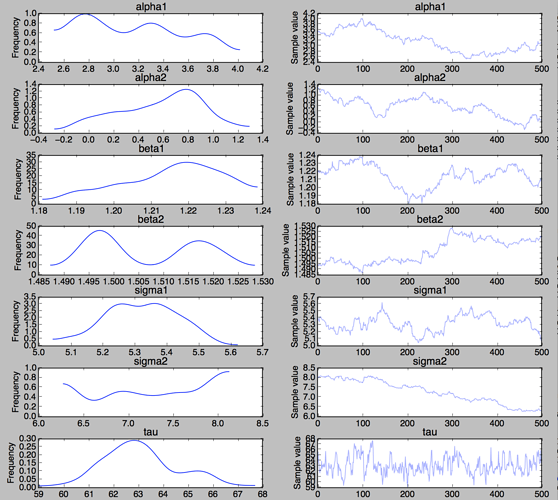
The w you provided in the python code is not the same as the R code generated.

Well spotted. I must have posted an old version of the R. I edited the question so that the data is the same for both R / Stan and Python. But my question remains: why does PyMC3 give such a poor answer?

hmm, seems even with the right data the default sampling is not performing well - the starting value estimated from ADVI is way off compare to MAP. @ferrine thoughts?

The difference between stan and pymc3 is due to how they initialize the mass matrix. The mass matrix allows nuts to make steps of different sizes for each variable, so for example the step size for mu2 should be much smaller than that for tau, since the posterior variance is much smaller in that direction.
Stan uses the warmup samples to adapt the step sizes, and pymc3 uses advi. In this particular example advi gives hideous estimates, which makes life hard for nuts. As the mass matrix doesn’t match the posterior variance at all, it needs to do very small steps, and to cover the same distance it has do to very many of those for each trajectory. It stops doing that after 2 ^ max_treedepth steps however and prints a warning instead. You end up with highly correlated samples.

I think what breaks advi in this model is that the posterior density is not continuous. (And this also makes life harder for nuts as well). Instead of using a hard switchpoint you could for example use a sigmoid to choose the parameter values:

with chg_model:
    # Priors for unknown model parameters
    alpha1 = pm.Normal('alpha1', mu=0, sd=10)
    alpha2 = pm.Normal('alpha2', mu=0, sd=10)
    beta1  = pm.Normal( 'beta1', mu=0, sd=10)
    beta2  = pm.Normal( 'beta2', mu=0, sd=10)
    sigma1 = pm.HalfNormal('sigma1', sd=10)
    sigma2 = pm.HalfNormal('sigma2', sd=10)

    tau = pm.Uniform('tau', lower=0, upper=len(w) + 1)
    weight = tt.nnet.sigmoid(2 * (x - tau))

    alpha = weight * alpha2 + (1 - weight) * alpha1
    beta = weight * beta2 + (1 - weight) * beta1
    sigma = weight * sigma2 + (1 - weight) * sigma1

    # Expected value of outcome
    mu = alpha + beta * x

    # Likelihood (sampling distribution) of observations
    Y_obs = pm.Normal('Y_obs', mu=mu, sd=sigma, observed=w)

The same thing should help stan as well, as the incontinuities are a problem for nuts, too.
(btw, it might be better to model the first parameter and the difference between the first and the second instead…)

After this change it seems to work fine:

Funnily enough I just pushed a pull request for pymc3 for dynamic mass matrix adaptation after advi yesterday. This isn’t really ready yet, but this seems to fix it as well: https://github.com/pymc-devs/pymc3/pull/2327

@idontgetoutmuch btw, in the stan model you probably shouldn’t use uniform that way. It’s better to just use real<lower=0, upper=N+1> in the parameters section. That way it can use a transformed version of your tau internally to make sure your model has support on R^n.

Excellent! That works for me too. I guess I am too used to being able to use discontinuities via diffusions which smooth them out.

For ADVI, I guess you use the approach here: https://arxiv.org/pdf/1506.03431.pdf?

I am now wondering about the trade offs of using ADVI Vs burn in but maybe that’s another question.

Thanks - I will do so.

Do open another thread - I think these are very interesting discussions and will help how we further improve PyMC. :wink:

Can you share how you found the starting value with a) ADVI and b) MAP?

You can used pm.sampling.init_nuts:

with model:
    #MAP
    start_map, nuts_step = pm.sampling.init_nuts(init='MAP')
    #ADVI
    start_advi, nuts_step = pm.sampling.init_nuts(init='ADVI')

where nuts_step is the nuts_sampler: pymc3.step_methods.NUTS.

You can also do it via using the specific function:

with model:
    #MAP
    start = pm.find_MAP()
    #ADVI
    approx = pm.fit(n=20000, method='advi', 
            obj_optimizer=pm.adagrad_window
        )  # type: pm.MeanField
    start = approx.sample(draws=1)[0]
2 Likes

Writing it like that makes it pretty clear that we should deprecate pm.find_MAP() and add a pm.fit(method='MAP').

So making pm.fit a general wrapper for Bayesian optimization?

Right, exactly. @ferrine does that fit into the fit api?

Fit is supposed to return Approximation instance. Map can be wrapped up with Empirical as well and return consistent type

I really appreciate the Idea to add step methods to fit and refactor the whole model to get the only function for calling Thomas Bayes’ help