Correctly applying switchpoint model?

[Gon_F]

So, I was interested in learning how to model switchpoints, and after reading some discussions (some links here, here, and here), I decided to jump into them with Pymc3.

After playing around a bit, I have a few questions (mostly to do with improving inference), that I would like to ask, and that I hope the very helpful community here will offer some suggestions with.

1. Data
   The data I created is a sine wave with basic normal noise at all times, with an upward squared trend coming in at the halfway point. Here is a picture,

, with the generating code,

# First, regular sine wave + normal noise
x = np.linspace(0,40, num=300)
noise1 = np.random.normal(0,0.3,300)
y = np.sin(x) + noise1

# Second, an upward trending starting halfway, with its own normal noise as well
temp = x[150:]
noise2 = 0.004*temp**2 + np.random.normal(0,0.1,150)
y[150:] = y[150:] + noise2

plt.plot(x, y)

And the first dummy model that I trained on this dataset, to see how it fared, was

y = \beta_0 + \beta_1\sin x + \beta_2x \ ,

and I can see that it captured the oscillation, as well as upward trend, well enough for such a mis-specified model.

(this graph is generated from my ad hoc posterior predictive checks)

2. 1st Switchpoint model
   Now, unto my real model. I proceeded to create an ideal model to see how well the switchpoint will be calculated.

   def model_factory1(X, Y):
   
       with pm.Model() as switchpoint_model:
   
           # Discrete uniform prior for the switchpoint
           switchpoint = pm.DiscreteUniform('switchpoint', lower=X.min(), upper=X.max(), testval=10)
    
           # Priors 
           beta1_offset = pm.Normal('beta1_offset')
           beta1 = pm.Deterministic("beta1", beta1_offset * 3)
    
           beta2_offset = pm.Normal('beta2_offset')
           beta2 = pm.Deterministic("beta2", beta2_offset * 3)
    
          intercept_offset = pm.Normal('intercept_offset', mu=0, sd=1)
          intercept = pm.Deterministic("intercept", intercept_offset * 3)
   
          std = pm.HalfNormal('std', sd=5)
   
          # Likelihood
          part1 = intercept + pm.math.dot(pm.math.sin(X), beta1)
            
          part2 = intercept + pm.math.dot(pm.math.sin(X), beta1) + \
                              pm.math.dot(pm.math.sqr(X), beta2)
            
          model = pm.math.switch(switchpoint >= X, part1, part2)
   
          y_lik = pm.Normal('y_lik', mu=model, sd=std, observed = Y)
   
       return switchpoint_model
   

Generating my traces, three times with three different settings (for robustness):

with model_factory1(x_shared, y_shared) as model:
     first_switchpoint_trace = pm.sample(cores=4)
     second_switchpoint_trace = pm.sample(cores=4, draws=3000, tune=3000)
     third_switchpoint_trace = pm.sample(init='advi', chains=8, cores=4, draws=3000,                tune=3000, n_init=30000)

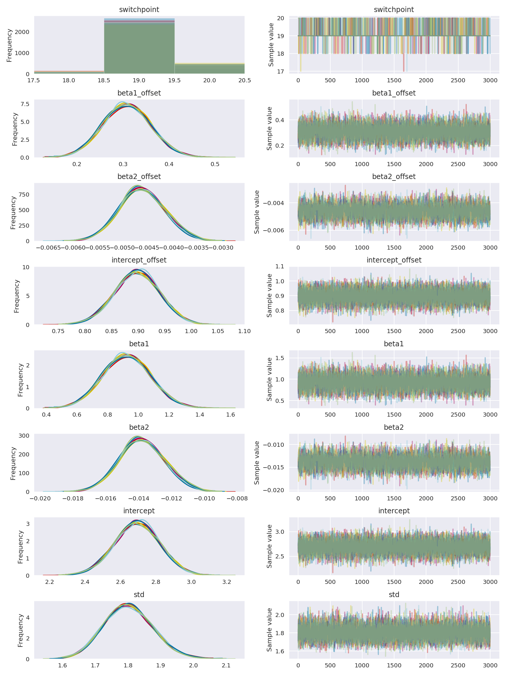
The results that I get are somewhat disheartening: the traceplots are all over the place, and none of them infer the correct switchpoint moment (the 150th data point, or x = 20), and yet the graphs made using my posterior predictive plots all look almost correct?

In addition, the first and last traces show huge chain divergence (which is confusing, since these represent both the easiest and hardest to compute chains), because, I imagine, the switchpoint nature of the model confuses some of the chains sometimes?

The traceplots:

PPC Graphs (all the same):

3. 2nd switchpoint model

For my 2nd Switchpoint model, I basically just followed junpenglao’s recommendation in the FAQ on using a sigmoid function, instead of pm.math.switch(), to make the sampler’s life easier when inferring the switchpoint (which is interesting).

The new code:

def model_factory2(X, Y):
    
    with pm.Model() as switchpoint_model:

        # Discrete uniform prior for the switchpoint
        switchpoint = pm.DiscreteUniform('switchpoint', lower=X.min(), upper=X.max(), testval=10)
        
        # Priors 
        beta1_offset = pm.Normal('beta1_offset')
        beta1 = pm.Deterministic("beta1", beta1_offset * 3)
        
        beta2_offset = pm.Normal('beta2_offset')
        beta2 = pm.Deterministic("beta2", beta2_offset * 3)
        
        intercept_offset = pm.Normal('intercept_offset', mu=0, sd=1)
        intercept = pm.Deterministic("intercept", intercept_offset * 3)

        std = pm.HalfNormal('std', sd=5)

        # Likelihood
        part1 = intercept + pm.math.dot(pm.math.sin(X), beta1)
                
        part2 = intercept + pm.math.dot(pm.math.sin(X), beta1) + \
                            pm.math.dot(pm.math.sqr(X), beta2)
          
        ## New code      
        weight = tt.nnet.sigmoid(2 * (X - switchpoint))
        model = weight * part1 + (1 - weight) * part2    
        
        y_lik = pm.Normal('y_lik', mu=model, sd=std, observed = Y)
    
    return switchpoint_model

The new traceplots now are much better, from the switchpoint location perspective (they are all generally close to x=20), but now my PPC’s looks absolutely mangled and terrible, and I cannot account for how this happened.

(hurray for posterior-predictive checks telling you if your model makes sense?)

With the abominable PPC:

3. Conclusion
   Basically, I’m coming away from this with two questions, which I hope much more experienced modelers can elaborate on.

   1. Despite the traceplots showing the correctly estimated switchpoint for the second model, (because the estimation method was better), why is the PPC so bad?

   2. Why do some of my chains show multiple hills, even though none of he variables are supposed to have different forms on different sides of the switchpoint (but rather, one variable is just added on one side of the switchpoint)?

I will appreciate any discussion and tips, and try to report on any progress made on my end.

[chartl]

There are tiny, tiny issues. Most fundamentally, because switchpoint is discrete, MH is used to sample it. This requires a large amount of tuning to explore the space. When you don’t use enough you get what you observed: MH hasn’t spent enough time bouncing around to find the optimal.

For MH i tend to use:

burn_in=10000
tune=5000
with pm.Model() as model:
  ...
  trace = pm.sample(1000, tune=tune + burn_in, chains=8, cores=3)

The second (tiny tiny) issue is with

model = pm.math.switch(switchpoint >= X, part1, part2)

This should read

model = pm.math.switch(tt.gt(switchpoint, X), part1, part2)

The third issue is with

std = pm.HalfNormal('std', sd=5)

This puts a lot of weight on error variances that exceed the range of the data. Using a more informative prior like

std = pm.HalfNormal('std', sd=0.5)

makes a huge difference in both cases.

With these three changes model 1 appears to work just fine:

and with confidence region:

y_mean = np.mean(ppc['y_lik'], 0)
y_u95 = np.percentile(ppc['y_lik'], 97.5, axis=0)
y_u05 = np.percentile(ppc['y_lik'], 2.5, axis=0)
plt.plot(X, y_mean)
plt.plot(X, y_u95, color='red')
plt.plot(X, y_u05, color='red')

Edit:

Oh and for model 2, I think the sigmoid weights are reversed:

    w = tt.nnet.sigmoid(2*(X-switchpoint))
    model = (1-w)*part1 + w*part2

  model = w*part1 + (1-w)*part2

[chartl]

By the way, it’s possible to avoid MH while simultaneously adding some intuition that the change-point will be somewhere “in the middle” of the trend, by using a scaled Beta (nb the hyperprior is enormously helpful for speeding up sampling):

with pm.Model() as switchpoint_model_noMH:
    # Scaled beta mixture "somewhere in the middle" prior
    a = pm.HalfNormal('a_hp', 3.)
    b = pm.HalfNormal('b_hp', 3.)
    sp_latent = pm.Beta('sp_latent', a, b)
    switchpoint = pm.Deterministic('switchpoint', X.min() + (X.max() - X.min()) * sp_latent)

    # Priors 
    beta1_offset = pm.Normal('beta1_offset')
    beta1 = pm.Deterministic("beta1", beta1_offset * 3)
 
    beta2_offset = pm.Normal('beta2_offset')
    beta2 = pm.Deterministic("beta2", beta2_offset * 3)
 
    intercept_offset = pm.Normal('intercept_offset', mu=0, sd=1)
    intercept = pm.Deterministic("intercept", intercept_offset * 3)

    std = pm.HalfNormal('std', sd=0.5)

    # Likelihood
    part1 = intercept + pm.math.dot(pm.math.sin(X), beta1)
         
    part2 = intercept + pm.math.dot(pm.math.sin(X), beta1) + \
                        pm.math.dot(pm.math.sqr(X), beta2)
         
    #model = pm.math.switch(tt.gt(switchpoint, X), part1, part2)
    w = tt.nnet.sigmoid(2*(X-switchpoint))
    model = (1-w)*part1 + w*part2

    y_lik = pm.Normal('y_lik', mu=model, sd=std, observed = Y)
    trace = pm.sample(1000, init='advi+adapt_diag', tune=tune + burn_in, chains=4, cores=3)
    ppc = pm.sample_posterior_predictive(trace, 1000)