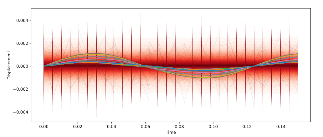
Hey! So, I’ve been tinkering with modeling the output of a FEM Model using GPs with the dimensions of the GP being time and a series of parameters which I intent to study. So long I’ve had some success when modelling a previous model which had only two dimensions (time and one parameter representing linear dampening). Now I’m running into some issues when modeling the output of another model which has linear dampening and a stiffness parameter as it’s inputs, the problem can be seen in the following plot where the GP samples are in red and the output from the FEM are the colored lines.
The code used to produce the GP samples is the following:
with pm.Model() as model:

    mu_EI = pm.HalfCauchy('mu_EI', beta = 5)

    sd_EI = pm.HalfCauchy('sd_EI', beta = 5)

    mu_AMALPHA = pm.HalfCauchy('mu_AMALPHA', beta = 5)

    sd_AMALPHA = pm.HalfCauchy('sd_AMALPHA', beta = 5)

    ℓ = pm.Normal('ℓ',

                    mu = mean_freqs.mean(),

                    sigma= 0.1) #A more precise period means we will be copying the GP!

    lenght_scale_EI = pm.TruncatedNormal('lenght_scale EI', lower = 0, upper = 10000,

                                mu = mu_EI,

                                sigma=sd_EI)
    lenght_scale_AMALPHA = pm.TruncatedNormal('lenght_scale_AMALPHA', lower = 0, upper = 10000,

                                        mu = mu_AMALPHA,

                                        sigma=sd_AMALPHA)

    η = pm.HalfCauchy("η", beta=5)

    cov = η**2 * pm.gp.cov.ExpQuad(3,

                         ls = [ℓ, lenght_scale_AMALPHA, lenght_scale_EI])

    σ = pm.HalfNormal("σ", sigma=0.1)

    gp = pm.gp.MarginalSparse(cov_func=cov, approx="FITC")

    input_u = pm.gp.util.kmeans_inducing_points(10, input_1)

    y_ = gp.marginal_likelihood(

        "y", X=input_1, Xu=input_u, y=studies.flatten(), noise=σ)

    time_new = np.linspace(0, max_samples * 1/200, num=max_samples)

    EI_cont = np.tile(EI, max_samples_params)

    _AMALPHA_cont =  np.tile(8.7e-05, max_samples_params)

    input_2 = pm.math.cartesian(

        time_new[:, None], _AMALPHA_cont[:, None], EI_cont[:, None])

    f_pred = gp.conditional('f_pred', input_2)

    pred_samples = pm.sample_posterior_predictive(

        trace=first_dataset, var_names=['f_pred'])
As seen in the code the samples are for constant values of both parameters which means the rest of the lines of the plot are mostly for comparison.
Is there any good modeling practice to avoid this behaviour? Am I commiting any silly mistake?
Thanks in advance!