Help model structure

Hello PyMC community !

For my thesis, I am trying to predict the performance of a company 5 years after it had a share buyback announcement. I am using as a prior to my Bayesian model the empirical performance of companies that had a share buyback, and I update the prior based on the proportion of the market capitalization that the share buyback represent, using the empirical data of company that had similar share buyback proportion.

However, the prediction obtained by my model does not make sense based on my empirical data, and I have been searching for the problem since few days now without finding the reason. Therefore, I was hoping to get some help here.

Here is my code:

#since my data is in the range of [-1.00:75.00], where -1.00 represent -100% and 1.5 represent 150%, I
#shifted it to have it positive and higher than 1.00 so I can apply log-transformation
shift = 2.01 
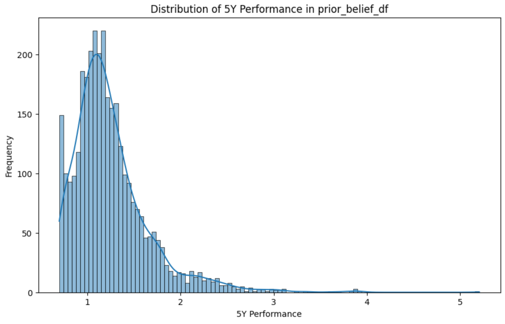
prior_belief_df = bb_df.groupby('company_ciqid')['5Y_performance'].mean().reset_index()
prior_belief_df.dropna(subset=['5Y_performance'], inplace=True)
prior_belief_df['5Y_performance_shifted'] = prior_belief_df['5Y_performance'] + shift

intervals = [0.00, 0.01, 0.03, 0.05, 0.15]#threshold considered for "marketcap_percentage"

X_aggregated = []
Y_aggregated = []

for lower_bound in intervals:
    filtered_df = bb_df[bb_df['marketcap_percentage'] >= lower_bound].copy()
    
    filtered_df['5Y_performance_shifted'] = filtered_df['5Y_performance'] + shift
    log_grouped_means = np.log(filtered_df.groupby('company_ciqid')['5Y_performance_shifted'].mean()).reset_index()

    X_aggregated.extend([lower_bound] * len(log_grouped_means))
    Y_aggregated.extend(log_grouped_means['5Y_performance_shifted'].values)


X = np.array(X_aggregated)
X_squared = X**2
Y = np.array(Y_aggregated)
log_5Y_performance = np.log(prior_belief_df['5Y_performance_shifted'])
global_log_median_performance = np.median(log_5Y_performance)
global_log_std_performance = np.std(log_5Y_performance)

with pm.Model() as model:
    #priors parameters using log-normal distribution
    alpha = pm.Lognormal('alpha', mu=global_log_median_performance, sigma=global_log_std_performance)
    beta = pm.Normal('beta', mu=0.01, sigma=0.005)  
    gamma = pm.Normal('gamma', mu=-0.005, sigma=0.0025)  
    sigma = pm.HalfNormal('sigma', sigma=1)

    #expected value of outcome, including the quadratic term
    log_mu = alpha + beta * X + gamma * X_squared

    #likelihood (sampling distribution) of observations
    Y_obs = pm.Lognormal('Y_obs', mu=log_mu, sigma=sigma, observed=Y)

    #model fitting
    trace = pm.sample(1000) 
def predict_performance(marketcap_percentage, trace, return_ci=True, ci_level=0.95):
    """
    Parameters:
    - marketcap_percentage: float, the marketcap percentage for which to predict performance.
    - trace: the trace object obtained after MCMC sampling.
    - return_ci: bool, whether to return credible intervals for the predictions.
    - ci_level: float, the confidence level for the credible interval (default is 95%).

    Returns:
    - A dictionary containing the predicted performance and, optionally, credible intervals.
    """
    #prepare new input data
    X_new = np.array([marketcap_percentage])
    X_squared_new = X_new ** 2
    
    #extract the posterior samples for the model parameters
    alpha_samples = trace.posterior["alpha"].values.flatten()
    beta_samples = trace.posterior["beta"].values.flatten()
    gamma_samples = trace.posterior["gamma"].values.flatten()
    
    #compute the expected log performance for the new input
    log_mu_new = np.mean(alpha_samples) + np.mean(beta_samples) * X_new + np.mean(gamma_samples) * X_squared_new
    
    #transform predictions back to original scale
    performance_pred = np.exp(log_mu_new) - shift  

    if return_ci:
        performance_samples = np.exp(alpha_samples[:, None] + beta_samples[:, None] * X_new + gamma_samples[:, None] * X_squared_new) - shift
        ci_lower, ci_upper = np.percentile(performance_samples, [(1 - ci_level) / 2 * 100, (1 + ci_level) / 2 * 100], axis=0)
    else:
        ci_lower, ci_upper = None, None
    
    result = {
        'predicted_mean_performance': performance_pred[0],  # Unpack the single value
        'credible_interval': (ci_lower[0], ci_upper[0]) if return_ci else None
    }
    
    return result
prediction = predict_performance(marketcap_percentage = 0.10, trace = trace)
print(prediction)

I obtain as result “{‘predicted_mean_performance’: -1.0041700801651028, ‘credible_interval’: (-1.0063240928821156, -1.0015744422770478)}”.

Base on my empirical data, the median performance of company with “marketcap_percentage” of 0.10 or more is 0.17, while the mean is 1.32. Therefore, non only the result is far from the empirical data, but it is also nonsense since a company can’t perform lower than -100%.

I would be more than happy if somebody tried to help me in finding what is wrong. Let me know if you need more information :nerd_face:

I just glanced over all the code; my first impression is that you should replace the predict_performance function with some kind of posterior predictive sampling. I’d make X into a pm.MutableData, then compute X_squared from it inside your model. After sampling you can use pm.set_data together with pm.sample_posterior_predictive. Example workflow here. From here you can inspect the samples and compute whatever summary statistics you’re interested in. This will be much less error prone than re-implementing the model in numpy and hoping for the best (i’m guilty of using this approach).

You should also check that the posterior predictives from your model make sense before you start the out-of-sample checks. At minimum it would rule out if the problem is in your model or your prediction workflow.

Thank you Jesse for taking the time to help, it’s really appreciated!
Perfect, the notions around it are still a little bit blurry to me, but it seems to make sense what you are suggesting. I will try it tomorrow morning!

This tutorial will also be nice to look at, it explains how to use data containers, and has an example of using pm.set_data for doing out-of-sample predictions towards the end.

Super, I’ll give it a look also !

I believe the problem stems from the model structure. I will try to give a quick concise explanation of my situation, so the readers have a better understanding.
I want to prediction the variable “5Y_performance”, which correspond to the performance of a company after it had a share buyback announcement. The empirical data range is [-1:175]. The prior of the model is the aggregated empirical data of performance of companies that had a share buyback announcement. I update the prior by using the information from the column “marketcap_percentage”, corresponding the the proportion of the share buyback.

The distribution of the untransformed data looks like this:

While the log-normal distribution looks like this (with a shift of 3.01 to have the data positive):

The structure of the Bayesian model looks like the following:

#since my data is in the range of [-1.00:175.00], where -1.00 represent -100% and 1.5 represent 150%, I
#shifted it to have it positive and higher than 1.00 so I can apply log-transformation
shift = 3.01
prior_belief_df = bb_belief_xs.groupby('company_ciqid')['5Y_performance'].mean().reset_index()
prior_belief_df.dropna(subset=['5Y_performance'], inplace=True)
prior_belief_df['5Y_performance_shifted'] = prior_belief_df['5Y_performance'] + shift

intervals = np.arange(0.00, 0.16, 0.01)

X_aggregated = []
Y_aggregated = []

for lower_bound in intervals:
    filtered_df = bb_belief_xs[bb_belief_xs['marketcap_percentage'] >= lower_bound].copy()
    filtered_df.dropna(subset=['5Y_performance'], inplace=True)

    filtered_df['5Y_performance_shifted'] = filtered_df['5Y_performance'] + shift

    log_grouped_means = np.log(filtered_df.groupby('company_ciqid')['5Y_performance_shifted'].mean()).reset_index()

    X_aggregated.extend([lower_bound] * len(log_grouped_means))
    Y_aggregated.extend(log_grouped_means['5Y_performance_shifted'].values)


X = np.array(X_aggregated)
Y = np.array(Y_aggregated)


log_5Y_performance = np.log(prior_belief_df['5Y_performance_shifted'])
global_log_median_performance = np.median(log_5Y_performance)
global_log_std_performance = np.std(log_5Y_performance)

with pm.Model() as model:

    X_data = pm.MutableData("X_data", X)

    alpha = pm.Lognormal('alpha', mu=global_log_median_performance, sigma=global_log_std_performance) 
    beta = pm.Normal('beta', mu=0.01, sigma=0.05)
    sigma = pm.HalfNormal('sigma', sigma=0.05) 

    log_mu = alpha + beta * X_data

    #likelihood (sampling distribution) of observations
    Y_obs = pm.Lognormal('Y_obs', mu=log_mu, sigma=sigma, observed=Y) 

    trace = pm.sample(1000, return_inferencedata=True)

with model:
    #generate posterior predictive samples
    posterior_predictive = pm.sample_posterior_predictive(trace)

The following code gives gives me the distribution of the observed data vs predicted data:

predicted_data = posterior_predictive.posterior_predictive["Y_obs"].values.flatten()

sample_size = 100000

predicted_data_sample = np.random.choice(predicted_data, size=sample_size, replace=False)

observed_data = Y

plt.figure(figsize=(10, 5))

sns.kdeplot(observed_data, color="blue", label="Observed Data")

sns.kdeplot(predicted_data, color="red", alpha=0.5, label="Predicted Data")

plt.title('Observed vs Predicted Data KDE')

plt.legend()

plt.show()


image

The residuals distribution looks like the following:

As we can see, the distribution of the predicted data seems to not be to different from the observed data, or I might be wrong since I am not experienced on the matter. However, the prediction that I obtain has a median always about 50% higher than the one from my empirical data, while the means changes just slightly when using a different “marketcap_percentage”, while my empirical data the means change substantially when playing with this parameter.

Here is the code used to make the prediction. It might not be correct:

#marketcap_percentage input to predict
new_X_values = np.array([0.15])

with model:
    pm.set_data({"X_data": new_X_values})

    #generate posterior predictive samples with updated X
    posterior_predictive = pm.sample_posterior_predictive(trace)

#access the posterior_predictive group directly
predicted_samples = posterior_predictive.posterior_predictive["Y_obs"]
predicted_samples_flat = predicted_samples.values.flatten()

reversed_exp = np.exp(predicted_samples_flat)
reversed_original = reversed_exp - shift

predicted_mean_original = np.mean(reversed_original)
predicted_median_original = np.median(reversed_original)

print("Mean of Predicted Y_obs in Original Scale:", predicted_mean_original)
print("Median of Predicted Y_obs in Original Scale:", predicted_median_original)

I would like to have the opinion of somebody experienced to understand what I am doing wrong.