How can one bring in predictive variables to a time series model?

Hello,

I’m following this tutorial, Air passengers - Prophet-like model — PyMC3 3.11.5 documentation to help with a time series problem at work.

My question is, has anyone done a prophet-like model or any time series model and added other predictive variables to help with predicte lift?

If so, what would this look like in terms of model code?

In the prophet framework, you can include additional variables exactly as normal. The benefit of Prophet is that it dispenses with the complicated Cox-Box statistical framework and just treats time series as a curve fitting exercise. The trend is just a piecewise linear function, and the season is just some trig functions. So there’s really nothing stopping you from just adding additional variables to the regression, but you need to be on guard against confounding between the trend and seasonal terms, and these additional terms. For example, if there is a trend or seasonal term in your explanatory variables, parameter estimates will not be identified.

Now, if you want inter-temporal dynamics (ARIMA terms), things get more complex, see this note by Rob Hyndman about how to include exogenous variables in the Cox-Box framework (SARIMAX). SARIMAX is not trivial in PyMC; one of the older hands will need to chime in if you are interested in that.

Here is a code estimating consumption based on the money supply using a Prophet-like setup. The example comes by way of the Statsmodel.api SARIMAX documentation. I’m on PyMC3, but everything in this snippet should be identical in PyMC4, just replace the theano import with aesara.

import pandas as pd
import requests
from io import BytesIO

import pymc3 as pm
import numpy as np
from theano import tensor as tt

from sklearn.preprocessing import StandardScaler

# Load data
friedman2 = requests.get('https://www.stata-press.com/data/r12/friedman2.dta').content
data = pd.read_stata(BytesIO(friedman2))
data.set_index('time', inplace=True)
data.index.freq = "QS-OCT"

# Slice and scale
scaler = StandardScaler()

data_slice = slice('1959', '1981')
use_data = data.loc[data_slice, ['consump', 'm2']].copy()

use_data.loc[:, :] = scaler.fit_transform(use_data.values)

y = use_data['consump'].copy()
X = (use_data.m2
        .to_frame()
        .assign(constant = 1)
        .loc[data_slice, :])

# Set up Prophet features
n_changepoints = 5
N = 3

def make_fourier_features(t, P, N=3):
    inner = 2 * np.pi * (1 + np.arange(N)) * t[:, None] / P
    return np.c_[np.cos(inner), np.sin(inner)]


#Coords for the PyMC model
time_idxs, times = pd.factorize(y.index)
time_idxs = time_idxs.astype(float)

# Trend matrix
s = np.linspace(0, max(time_idxs), n_changepoints + 2)[1:-1]
A = (time_idxs[:, None] > s) * 1.

break_idxs = np.apply_along_axis(lambda x: np.flatnonzero(x)[0], axis=0, arr=A)
break_dates = [f'{x.year}Q{x.quarter}' for x in times[break_idxs]]

# Make fourier features, P=24 to match a six year business cycle in quarterly data
X_fourier = make_fourier_features(t=time_idxs, P=24, N=3)

X_exog = X['m2'].copy()


coords = dict(
    time = times,
    fourier_features = [f'{func}_{i+1}' for func in ['cos', 'sin'] for i in range(N)],
    break_dates= break_dates,
    exog = ['m2']
)

# Model
with pm.Model(coords = coords) as freidman_model:
    k = pm.Normal('base_trend', mu = 0.0, sigma = 1.0)
    m = pm.Normal('base_intercept', mu = 0.0, sigma = 1.0)
    
    delta = pm.Normal('trend_offsets', mu=0.0, sigma=1.0, dims=['break_dates'])
    beta_seasonal = pm.Normal('beta_seasonal', mu=0.0, sigma=1.0, dims=['fourier_features'])
    beta_exog = pm.Normal('beta_exog', mu=0.0, sigma=1.0, dims=['exog'])
    
    growth = (k + tt.dot(A, delta))
    offset = m + tt.dot(A, (-s * delta))
    
    trend = growth * time_idxs + offset
    seasonality = tt.dot(X_fourier, beta_seasonal)
    exogenous = X_exog.values * beta_exog
    
    mu = trend + seasonality + exogenous
    sigma = pm.HalfNormal('sigma', sigma=1.0)
    
    likelihood = pm.Normal('y_hat',
                           mu    = mu,
                           sigma = sigma,
                           observed = y)

# Sample
with freidman_model:
    freidman_trace = pm.sample(cores= 6,
                              target_accept=0.9,
                              return_inferencedata=True)

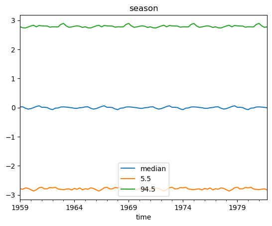
Here are the results:

The fit looks good, but this is a very spurious regression and we’re basically just fitting to the (mostly linear) trend. If we were doing real modeling work, you would want to render consumption stationary before doing any of this. More importantly, the M2 money supply is essentially a second trend term. As a result, the estimates for base_trend, base_intercept, trend_offsets, and beta_exog are going to be biased. I re-ran the model taking two differences of the money supply (rendering it stationary via eyeball test, I didn’t bother to do something more formal). Here are plots comparing some posterior estimates:

Naively including the M2 money supply as an explanatory variable before checking it was stationary not only skunked our estimates of the trend and intercept, but it also flipped the sign of the effect of monetary policy on consumption. Obviously we would need to do many more tests to make sure this model is correctly specified. I certainly wouldn’t stake my reputation on it as-is.

So in conclusion, the Prophet framework is nice because you are just doing a standard linear regression using a piecewise linear trend and some fourier features as explanatory variables. This makes it easy to expand and include additional explanatory variables. Nevertheless, you can’t throw out all the stuff you learned in Time Series 101 just because you have a fancy model.

4 Likes

That has to be the best, most in depth answer I’ve ever received through private message.

Thank you for taking the time to thoroughly explain this.

One more question, only if you have time. A consultant suggested we use a typical time series stats model to forecast demand, then use other variables to try and model the residuals. Is this technique possible in a Bayesian framework or is it even needed?

My apologies if these are juvenile questions. I am coming from the insurance industry where I did zero time series models.

Thank you again for being so generous with your time.

Jordan

No worries, we’re all figuring this out together!

When you do a two-step model like the one the consultant suggested, you can always do algebraic substitution to simplify it into one model. If we’re forcasting y_t, we could write:

\begin{align}\hat{y}_t &= f(y_{t-1}, y_{t-1}, \dots) + \hat{\epsilon}_t \\ \hat{\epsilon}_t &= f(X) + \hat{\eta}_t \end{align}

Note that you can simply substitute the second equation into the first and you get a single model. There might be technical reasons why you would want to do it in 2 steps, but strictly speaking it’s not necessary.

Note, however, that coefficients on exogenous variables lose their usual meaning of "a one unit increase in X leads to a \beta increase in y_t if you first model the time series dynamics then model the exogenous variables. This is because y_{t-1} is also a function of f(X), so you have to work through the algebra. You can recover the usual parameters with a bit of work, but it’s something to be aware of. Depending on your use-case, you might or might not care. If you only care about optimizing a forecasting metric, this won’t matter, but you might also be interested in trying to make some causal inferences, in which case it does. The Rob Hyndman blog post I linked to above discusses this issue in more detail.

The advantage of the the way the consultant suggests is that the residuals of the time series regression should end up stationary and ready for modeling. If you do the exogenous-first method, you will likely need to do some preprocessing: taking logs or first differences at a minimum. It comes down to personal preference. Other things to look into are STL decomposition or X-ARMIA13-SEATS. These do automatic time series decomposition so you could run that first, then do your exogenous variable model on the residuals (STL has a lot of hyperparameters you might have to grid search over, but X13 is very automatic). Forcasting: Principals and Practice has a nice high-level overview of these methods, and both are available in Statsmodels.api.

You can definitely do the two-step process in a Bayesian framework, though I’ve admittedly never tried to set it up in PyMC. My naive approach would be to model \hat{y}_t as usual, then construct \epsilon_t = y_t - \hat{y}_t and set up a second likelihood with this epsilon as the observed variable and a mean of f(X). That might be dumb though, someone else can chime in.

Is this necessary? I have no idea. It depends on your use-case. The exogenous variables might be helpful in forecasting or they might not be. If I were you, I would run some tests in a SARIMAX framework and see what it looks like before I sank a lot of time into sitting around waiting for NUTS to sample. I’ve been shocked at how hard it is to improve on simple ARIMA baselines in time series forecasting.

2 Likes

Good morning @jessegrabowski

Would you mind sharing how you produced the top graph?

I just replaced the random variables in trend, seasonality, and exogenous with the mean of the posterior of their respective distributions, then did fill_between the 0.05 and 0.95 quantiles to get the confidence interval.

Thank you. I meant how do you pull out the entire graph from trend down to predicted.

The prediction is given by the sum of the components, mu = trend + seasonality + exogenous. So you just need to sample all the bits (k, m, delta, betas), compute trend, seasonality, and exogenous, get the mean and quantiles for each, then plot them. For the total it’s easiest to just use the posterior predictive samples (that way the observation noise will be included – i over looked this in my plots), but it’s a good sanity check to confirm the sum of the means of the components and the mean of the posterior predictive are the same.

When you’re breaking out your time indexes and break dates, is there a way to do it when you have the same date multiple times in the dataset? For example, when I have multiple dates for multiple items, I get the following error when running the below code:

time_idxs, times = pd.factorize(y.index)
time_idxs = time_idxs.astype(float)
break_idxs = np.apply_along_axis(lambda x: np.flatnonzero(x)[0], axis=0, arr=A)
break_dates = [f'{x.year}Q{x.quarter}' for x in times[break_idxs]]

Error

---------------------------------------------------------------------------
IndexError                                Traceback (most recent call last)
/tmp/ipykernel_3156/2837611204.py in <module>
      2 time_idxs = time_idxs.astype(float)
      3 break_idxs = np.apply_along_axis(lambda x: np.flatnonzero(x)[0], axis=0, arr=A)
----> 4 break_dates = [f'{x.year}Q{x.quarter}' for x in times[break_idxs]]

/opt/conda/lib/python3.7/site-packages/pandas/core/indexes/extension.py in __getitem__(self, key)
    277 
    278     def __getitem__(self, key):
--> 279         result = self._data[key]
    280         if isinstance(result, type(self._data)):
    281             if result.ndim == 1:

/opt/conda/lib/python3.7/site-packages/pandas/core/arrays/datetimelike.py in __getitem__(self, key)
    320         only handle list-likes, slices, and integer scalars
    321         """
--> 322         result = super().__getitem__(key)
    323         if lib.is_scalar(result):
    324             return result

/opt/conda/lib/python3.7/site-packages/pandas/core/arrays/_mixins.py in __getitem__(self, key)
    205         )
    206         key = check_array_indexer(self, key)
--> 207         result = self._ndarray[key]
    208         if lib.is_scalar(result):
    209             return self._box_func(result)

IndexError: index 60757 is out of bounds for axis 0 with size 1824

I tried running the following:

break_dates = [f'{x.year}M{x.month}' for x in times[break_idxs].unique()]

Python doesn’t like attaching a function onto that though.

Looks like times is the unique timestamps (there are 1824),. but A is repeated for all the (item, time) pairs. So when you ran my code to look for breakpoints, you ended up with 60,757 breaks.

The way I’ve done it, length of A, in your case, should be 1824, at least when setting things up at first. A should be n_timesteps x k_breakpoints. My example only had one time series, but if you have multiple, I would handle duplicating A for each item after you run this code.

Anyway this code just sets up nice labels for the coords, it’s not essential.

hi @jessegrabowski , im working on trying to rebuild the plots of the predicted vs true but having trouble computing trend, seasonality, and exogenous.

I’m able to compute the exogenous component, but cant figure out the dot products on the posterior – any help would be appreciated:

k = ppc_samples["base_trend"]
m = ppc_samples['base_intercept']
# , mu = 0.0, sigma = 1.0)

delta =ppc_samples['trend_offsets']
# , mu=0.0, sigma=1.0, dims=['break_dates'])
beta_seasonal =ppc_samples['beta_seasonal']

# , mu=0.0, sigma=1.0, dims=['fourier_features'])
beta_exog =ppc_samples['beta_exog'] 
# pm.Normal('beta_exog', mu=0.0, sigma=1.0, dims=['exog'])

exogenous = X_exog.values * beta_exog

offset = m + np.dot(A, (-s * delta))
growth = (k + np.dot(A, delta))


trend = growth * time_idxs + offset


seasonality = np.dot(X_fourier, beta_seasonal)

---------------------------------------------------------------------------
ValueError                                Traceback (most recent call last)
Input In [521], in <cell line: 14>()
     11 # pm.Normal('beta_exog', mu=0.0, sigma=1.0, dims=['exog'])
     13 exogenous = X_exog.values * beta_exog
---> 14 offset = m + np.dot(A, (-s * delta))
     15 growth = (k + np.dot(A, delta))
     18 trend = growth * time_idxs + offset

File <__array_function__ internals>:180, in dot(*args, **kwargs)

ValueError: shapes (92,5) and (6000,5) not aligned: 5 (dim 1) != 6000 (dim 0)

once i get those component series i can plot the means/confidence intervals as well as plot the summed series.

Thanks!

The error lists the shapes in the same order as the arguments of the function, which is helpful to debug these types of shape errors.

It’s telling you that the matrix A has shape (92,5), while the product (-s * delta) has shape (6000, 5). I guess 6000 is the sample dimension? In that case, you just need to transpose: (-s * delta).T, then the resulting dot will have shape (time, samples). You will need to keep in mind that samples is now the 2nd dimension, and you can transpose again if you prefer it on the first. It doesn’t matter which you choose, you just have to be consistent with all your computations so additions between the components line up.

1 Like

ah I see, cool thanks, after fixing those shape mismatches im able to get a similar output to ur charts but def not matching completely, this is still using the levels but the confidence intervals dont seem to match yours – did I compute them right?


def compute_bands(vals, levels=[5.5, 12.5, 25, 75, 87.5, 94.5]):
    def scoreatpercentile(vals, p):
        return [sp.stats.scoreatpercentile(temp,p) for temp in vals.T]
    perc = {p:scoreatpercentile(vals,p) for p in levels}
    median = np.median(vals, axis=0)
    perc["median"] = median
    return perc
k = ppc_samples["base_trend"]
m = ppc_samples['base_intercept']
# , mu = 0.0, sigma = 1.0)

delta =ppc_samples['trend_offsets']
# , mu=0.0, sigma=1.0, dims=['break_dates'])
beta_seasonal =ppc_samples['beta_seasonal']

# , mu=0.0, sigma=1.0, dims=['fourier_features'])
beta_exog =ppc_samples['beta_exog'] 
# pm.Normal('beta_exog', mu=0.0, sigma=1.0, dims=['exog'])

exogenous = X_exog.values * beta_exog

offset = m + np.dot(A, (-s * delta).T)

growth = (k + np.dot(A, delta.T))


trend = growth.T * time_idxs + offset.T


seasonality = np.dot(X_fourier, beta_seasonal.T).T

# growth = (k + tt.dot(A, delta))
mu = trend + seasonality + exogenous
pd.DataFrame(compute_bands(trend),index=y.index)[["median",5.5,94.5]].plot(title="trend")

pd.DataFrame(compute_bands(seasonality),index=y.index)[["median",5.5,94.5]].plot(title="season")

pd.DataFrame(compute_bands(exogenous),index=y.index).join(X["m2"])[["median",5.5,94.5,"m2"]].plot(title="exogenous")


pd.DataFrame(compute_bands(mu),index=y.index).join(y)[["consump","median",5.5,94.5]].plot(title="predicted")

and here are the images:

exog
predicted
season
trebd

Sorry for the slow response. Something is definitely off in your plots.

You’re re-running the Friedman model I guess? I think there might be some shape problems, but I couldn’t say. It also looks like you didn’t scale the data, I would always recommend doing that. Here is my code for the plots, note that az.extract_dataset puts the samples on the last index:

posterior = az.extract_dataset(freidman_trace, 'posterior')

exogenous = X_exog.values[:, None] * posterior.beta_exog.values
offset = posterior.base_intercept.values + np.dot(A, (-s[:, None] * posterior.trend_offsets.values))
growth = (posterior.base_trend.values + np.dot(A, posterior.trend_offsets.values))
trend = growth * time_idxs[:, None] + offset
seasonality = np.dot(X_fourier, posterior.beta_seasonal)

mu = trend + seasonality + exogenous 

# Make sure to draw from the predictive distribution for the predictions, don't just use mu
predictions = np.random.normal(loc=mu, scale=posterior.sigma.values)

fig, ax = plt.subplots(4, figsize=(14,9))
names = ['Trend', 'Seasonal', 'Exogenous', 'Predicted']
datas = [trend, seasonality, exogenous, predictions]
for axis, data, name in zip(fig.axes, datas, names):
    q05, q5, q95 = np.quantile(data, [0.05, 0.5, 0.95], axis=-1)
    axis.plot(X_exog.index, q5)
    axis.fill_between(X_exog.index, q05, q95, alpha=0.1)
    axis.set(title=name)

I’m not sure why there is more uncertainty in the trend component than in the predictions, but it looks like that even when I use pm.sample_posterior_predictive. Also not sure what I did for those original plots above, those confidence blobs around the seasonal component look crazy…

2 Likes

Thanks so much! Yes rerunning the Friedman model. Haha ye the CI I computed are deff crazy deff shape errors.