How do you formulate a `Latent` GP that is equivalent to the `Marginal` implementation?

[BioGoertz]

As part of a larger model, I’m trying to use the Latent GP implementation in an equivalent way to the Marginal GP implementation (i.e., white noise and Normal observation likelihood), but my attempt yields different results.

Imports

from scipy.spatial.distance import pdist
import pymc3 as pm
import numpy as np
import matplotlib.pyplot as plt

SEED=2020
rng = np.random.default_rng(SEED)

Toy Data

X = np.linspace(0.1,1,20)[:,None]
X = np.vstack([X,X+1.5])
X_ = X.flatten()
y = np.sin(2*np.pi*X_) + rng.normal(0,0.1,len(X_))
σ_fun = (0.1+2*(X_%1.5))/3
y_err = rng.lognormal(np.log(σ_fun),0.1)

y_obs_ = rng.normal(y,y_err,size=(5,len(y)))
y = y_obs_.mean(axis=0)
y_err = y_obs_.std(axis=0)
y_obs = y_obs_.T.flatten()
X_obs = np.tile(X.T,(5,1)).T.reshape(-1,1)
X_obs_ = X_obs.flatten()
idx = np.tile(np.array([i for i,_ in enumerate(X_)]),(5,1)).T.flatten()

Xnew = np.linspace(-0.25,3.25,100)[:,None]
Xnew_ = Xnew.flatten()
ynew = np.sin(2*np.pi*Xnew_)

plt.plot(X,y,'C0o')
plt.errorbar(X_,y,y_err*2,color='C0',ls='none')
plt.plot(X_obs,y_obs,'C1.')

Get lengthscale prior hyperparameters

def get_ℓ_prior(points):
    distances = pdist(points[:, None])
    distinct = distances != 0
    ℓ_l = distances[distinct].min() if sum(distinct) > 0 else 0.1
    ℓ_u = distances[distinct].max() if sum(distinct) > 0 else 1
    ℓ_σ = max(0.1, (ℓ_u - ℓ_l) / 6)
    ℓ_μ = ℓ_l + 3 * ℓ_σ
    return ℓ_μ, ℓ_σ

ℓ_μ, ℓ_σ = [stat for stat in get_ℓ_prior(X_)]

Marginal Likelihood Formulation

with pm.Model() as model_marg:
    ℓ = pm.InverseGamma('ℓ', mu=ℓ_μ, sigma=ℓ_σ)
    η = pm.Gamma('η', alpha=2, beta=1)
    cov = η ** 2 * pm.gp.cov.ExpQuad(input_dim=1,ls=ℓ)

    gp_marg = pm.gp.Marginal(cov_func=cov)

    σ = pm.Exponential('σ', lam=1)
    
    ml_marg = gp_marg.marginal_likelihood('ml_marg', X=X_obs, y=y_obs, noise=σ)

    mp_marg = pm.find_MAP()

Sample and Plot Posterior

with model_marg:
    mu_marg = gp_marg.conditional("mu_marg", Xnew=Xnew)
    samples_marg = pm.sample_posterior_predictive([mp_marg], var_names=['mu_marg'], samples=500)

mu_marg = samples_marg["mu_marg"].mean(axis=0)
sd_marg = samples_marg["mu_marg"].std(axis=0)

plt.plot(Xnew_,mu_marg,'C0')
plt.fill_between(Xnew_,mu_marg+2*sd_marg,mu_marg-2*sd_marg,facecolor='C0',alpha=0.5)
plt.plot(X_obs,y_obs,'C1.')
plt.title('"Marginal" GP Formulation')

MAP values

• ℓ: 0.43
• η: 2.51
• σ: 0.48
  

Latent Formulation

with pm.Model() as model_lat:
    ℓ = pm.InverseGamma('ℓ', mu=ℓ_μ, sigma=ℓ_σ)
    η = pm.Gamma('η', alpha=2, beta=1)
    σ = pm.Exponential('σ', lam=1)
    cov = η ** 2 * pm.gp.cov.ExpQuad(input_dim=1,ls=ℓ) + pm.gp.cov.WhiteNoise(sigma=0.001)

    gp_lat = pm.gp.Latent(cov_func=cov)
    mu = gp_lat.prior('mu', X=X_obs)
    
    lik_lat = pm.Normal('lik_lat', mu=mu, sd=σ, observed=y_obs)

    mp_lat = pm.find_MAP()

Sample and Plot Posterior

with model_lat:
    mu_lat = gp_lat.conditional("mu_lat", Xnew=Xnew)
    samples_lat = pm.sample_posterior_predictive([mp_lat], var_names=['mu_lat'], samples=500)

mu_lat = rep_samples["mu_lat"].mean(axis=0)
sd_lat = rep_samples["mu_lat"].std(axis=0)

plt.plot(Xnew_,mu_rep,'C0')
plt.fill_between(Xnew_,mu_lat+2*sd_lat,mu_lat-2*sd_lat,facecolor='C0',alpha=0.5)
plt.plot(X_obs,y_obs,'C1.')
plt.title('"Marginal" GP Formulation')

MAP values:

• ℓ: 0.46
• η: 5.21
• σ: 0.47
  

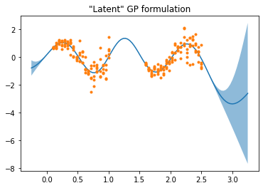
Interestingly, the MAP value on the variance scale η is very different between the two. The Marginal GP behaves more like I’d expect, with epistemic uncertainty growing rapidly outside the regions with observations. Any idea how I construct an equivalent to Marginal using the Latent impementation?

[bwengals]

I think MAP inference for the Latent model would be really tough to get to work, I would guess there are a lot of local minima with mu. Have you tried the NUTS sampler? I would hope that NUTS would give you matching results.

[BioGoertz]

So sampling with NUTS does give posterior modes that are more in line with the MAP estimate from the Marginal GP:

NUTS posterior:

• ℓ:
  • mean: 0.43
  • mode: 0.42
• η:
  • mean: 2.55
  • mode: 2.7
• σ:
  • mean: 0.49
  • mode: 0.49

Sampling over the whole trace (sample_posterior_predictive(trace,...)) does give a nearly-identical uncertainty profile to the Marginal GP:

However, if I understand correctly, the uncertainty shown there compounds uncertainty in the hyperparameters with uncertainty in the GP that results from any given set of hyperparameters. Sampling over the Marginal GP fit via MAP has no hyperparameter uncertainty, only uncertainty in the mean of the GP itself. It seems that a more apples-to-apples comparison is to sample over the Latent GP using the mean of each hyperparameter posterior as a fixed point (sample_posterior_predictive([trace_rep_l.posterior.mean(dim=['chain','draw'])],...)). That gives a curve similar to the result of Latent with find_MAP.

Am I maybe misunderstanding how sampling works in the Marginal implementation?

[bwengals]

I do think the most apples-to-apples comparison is to use NUTS to sample both Latent and the Marginal version. Then to get explicit samples of mu, use Marginal.conditional. I think here the hyperparameter and mu posteriors should all be the same.

I think what you are seeing using find_MAP are local minima. I think fixing the means of the hyperparameters and getting the same result on mu with NUTS is evidence towards this – that spot we are seeing in the plot must be a pretty high probability region (given those specific values of theta).

[BioGoertz]

Okay, here’s what confuses me. Sampling the Marginal GP over the full trace (a distribution of hyperparameters), sampling the Marginal GP at the trace mean (a single point), and sampling the Latent GP over the full trace all look very similar, whereas sampling the Latent GP at its trace mean is very different than the others. This is without predicting noise, so all uncertainty is epistemic.

I guess I don’t understand where the additional uncertainty in sampling Marginal at a single point “comes from”, as compared to sampling Latent at a single point.

[bwengals]

So for the first three, yeah they should all be exactly the same. Sampling from Marginal is exactly the same as sampling from Latent and then chucking out the f samples (marginalization). That’s why it got called Marginal. To recover f from Marginal, you do have to use .conditional, but the f is the same as the f you got from Latent and NUTS.

I think past that, doing things like fixing the mean of f (or any other parameter like the lengthscale or eta) and sampling the rest may give inconsistent results. I’m not sure what should be expected in those cases. It is interesting that the result is so similar to running find_MAP, but it may just be a coincidence. I suspect in this case that find_MAP didn’t find the actual MAP point, but a local maxima. I think the result you get by fixing the mean and then sampling kind of backs this up as that may be an “important” location in f space in this case, but I’m just speculating on this though.

Does that help explain things? Please let me know if it seems like I’m not getting what you’re saying.