Hi @jessegrabowski ,
I tried to make a minimal example of the project I’m working on.
I created two notebooks that make use of tide-gauge data downloaded from the permanent service for mean sea level (psmsl). It tries to fit a linear trend to the tide-gauges with an AR(1) residual (the trend represents the combination of sea-level rise and vertical land motion, which we do not try to disentangle here). That exercise was pretty useful in itself, but if you find the time to give it some thinking, I’d be most grateful ! Let me explain here (the notebooks are not or poorly commented).
First regarding what I was saying in previous posts, I was actually attempting to model the noise explicitly, which is vastly more resource-intensive to do, and has convergence issues, but presents a few advantages (mainly a) it’s easier to build a meaningful likelihood function, as the covariances are modelled directly, b) missing data are handled seemlessly). Now I’ll try to focus on modelling the noise implictly, as is done in the VAR example. The main issue I encounter are missing data in the multivariate case. So in the process the question shifted to specifically multivariate AR(1) to how to handle missing data in multiple dimensions. Maybe that should be another question focused on missing data, but for the sake of the discussion above, and for the focus on auto-correlated noise, I stay here for now. I sum-up the experiments in the notebook’s header. I find that
- In the univariate case, missing data are best handled by just removing the nan bits, or by using a masked array to impute the missing data (I’m not sure what’s happening in there though, using as a black box). Setting missing data to zero (in predicted value and in obs) seems to introduce biases (only on the noise variance in the univariate example, but also on the slope in the multivariate case). I also compare with explicitly modelling the noise, which is further off. Here the results:

- In the second notebook (further down), I solve for 14 tide gauges simultaneously. I use a simplified VAR modelling where cross-correlation only come from the noise (there are no cross-coefficients for auto-correlation). Below the summary figure compares three settings:
- uncorrelated noise with dropped nans (“uncorr drop”)
- uncorrelated noise with zeroed nans (“uncorr zeros”)
- correlated noise with zeroed nans (“corr”)
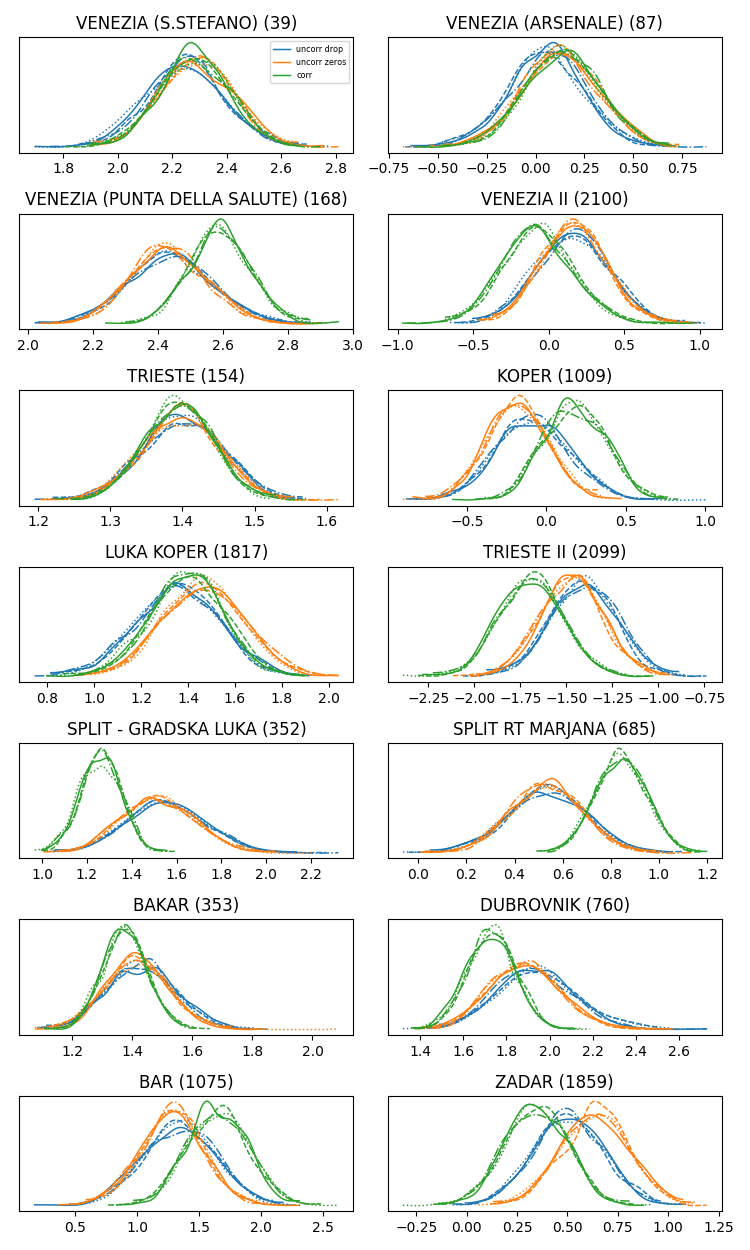
That seems to work alright but I am worried about missing data. There are at times small differences between dropped and zeroed nans in the uncorrelated case, and I worry that might impede a good estimate of the correlation between stations. Unfortunately, the masked array trick does not work in the multivariate case. I did attempt an equivalent of the “drop” case by constructing the full covariance matrix as cov = lkjcorr * stds * stds[None] and then using yearly observations MvNormal(..., mu=prediction[year, valid], cov=cov[valid, valid], observed=obs[year, valid]) but pymc does not seem to handle it (it compiles forever; not included in the toy notebook). The explicit noise modelling also took forever to run so I gave up here (I my real application it actually works in a reasonable time (15 min per 1000 draws per chain), albeit with a few divergences ~10 per 1000 samples).
That is it. I am not sure how easy/difficult that is to follow this, or whether that presents any interest to you in term of generality / applicability to other users. If I can make the examples more useful, please let me know.
I saw here that @fonnesbeck is knowledgeable about missing data. Maybe there is a way to handle the multivariate case as well?
Any hint would be much appreciated. Thanks.
EDIT: here the multivariate model in full:
import numpy as np
import pymc as pm
import pytensor.tensor as pt

# get the data
# ----------------
import urllib.request
import io
import pandas as pd

def fetch_psmsl(id):
    url = f"https://psmsl.org/data/obtaining/rlr.annual.data/{id}.rlrdata"
    with urllib.request.urlopen(url) as response:
       urlData = response.read()
    df = pd.read_csv(io.StringIO(urlData.decode()), sep=';', header=None, na_values=-99999)
    df.columns = ['year', 'value', 'flag', 'missing days']
    df['value'] -= 7000
    s = df.set_index('year')['value']
    s.name = id
    return s


stations = {'VENEZIA (S.STEFANO)': 39,
 'VENEZIA (ARSENALE)': 87,
 'VENEZIA (PUNTA DELLA SALUTE)': 168,
 'VENEZIA II': 2100,
 'TRIESTE': 154,
 'KOPER': 1009,
 'LUKA KOPER': 1817,
 'TRIESTE II': 2099,
 'SPLIT - GRADSKA LUKA': 352,
 'SPLIT RT MARJANA': 685,
 'BAKAR': 353,
 'DUBROVNIK': 760,
 'BAR': 1075,
 'ZADAR': 1859}

data = pd.DataFrame({id:fetch_psmsl(id) for id in stations.values()})

df = data
years = df.index.values
nt, n = df.shape

with pm.Model() as model:

    model.add_coord('year', years)
    model.add_coord('year_predicted', years[1:])
    model.add_coord('station', length=n)

    rho = pm.Normal('rho', dims='station')
    # sigma = pm.HalfNormal('sigma', 1, dims='station')
    sigma = pm.HalfNormal.dist(1, size=n)
    chol, _, _ = pm.LKJCholeskyCov('lkj', eta=1, sd_dist=sigma, n=n)
    intercept = pm.Normal('intercept', 0, 10, dims='station')
    slope = pm.Normal('slope', 0, 100, dims='station')

    trend = intercept[None] + slope[None]*(years[:, None]-1950)
    pm.Deterministic(f'trend', trend, dims=('year', 'station'))

    # Factor out missing values by setting predicted = observed = 0
    missing = np.isnan(df.values)
    obs = df.fillna(0).values

    ano = obs - trend
    ar_mean = ano*rho[None]
    pred = trend[1:] + ar_mean[:-1]

    mask_pred = missing[:-1]
    aligned_obs = obs[1:].copy()
    mask_obs = missing[1:]

    mask = mask_pred | mask_obs

    for j in range(n):
        i, = mask[:, j].nonzero()
        pred = pt.set_subtensor(pred[i, j], 0)
        aligned_obs[i, j] = 0

    # masking out missing data does not work in multiple dimensions
    # observed = np.ma.array(aligned_obs, mask=mask)
    observed = aligned_obs
    pm.Deterministic(f'trend_plus_armean', pred, dims=('year_predicted', 'station'))
    pm.ConstantData(f'obs', aligned_obs, dims=('year_predicted', 'station'))
    pm.Deterministic(f'ar_mean', ar_mean[:-1], dims=('year_predicted', 'station'))
    pm.MvNormal(f'tidegauge_obs', mu=pred, chol=chol, observed=observed, dims=('year_predicted', 'station'))

    idata = pm.sample()