How to decide on what priors distributions to use for parameters?

[Mojo_ild]

I am looking into pymc3 package where I was interested in implementing the package in a scenario where I have several different signals and each signal have different amplitudes.

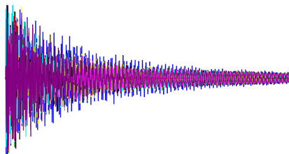
However, I was stuck in what type of priors I would need to use in order to implement pymc3 into it and likelihood distribution to implement. Scenario example is shown in the following picture

I tried to implement it here, but, every time I keep on getting bad initial energy. Error message can be found here:

pymc3.exceptions.SamplingError: Bad initial energy

Find my portion of the code below:

    ## Signal 1:
        with pm.Model() as model:
            # Parameters:
            # Prior Distributions:
            # BoundedNormal = pm.Bound(pm.Exponential, lower=0.0, upper=np.inf)
            # c = BoundedNormal('c', lam=10)
            # c = pm.Uniform('c', lower=0, upper=300)
            alpha = pm.Normal('alpha', mu = 0, sd = 10)
            beta = pm.Normal('beta', mu = 0, sd = 1)
            sigma = pm.HalfNormal('sigma', sd = 1)
            mu = pm.Normal('mu', mu=0, sigma=1)
            sd = pm.HalfNormal('sd', sigma=1)

            # Observed data is from a Multinomial distribution:
            # Likelihood distributions:
            # bradford = pm.DensityDist('observed_data', logp=bradford_logp, observed=dict(value=S1, loc=mu, scale=sd, c=c))
            # observed_data = pm.Beta('observed_data', mu=mu, sd=sd, observed=S1)
            observed_data = pm.Beta('observed_data', alpha=alpha, beta=beta, mu=mu, sd=sd, observed=S1)

        with model:
            # obtain starting values via MAP
            startvals = pm.find_MAP(model=model)

            # instantiate sampler
            # step = pm.Metropolis()
            step = pm.HamiltonianMC()
            # step = pm.NUTS()

            # draw 5000 posterior samples
            trace = pm.sample(start=startvals, draws=1000, step=step, tune=500, chains=4, cores=1, discard_tuned_samples=True)

            # Obtaining Posterior Predictive Sampling:
            post_pred = pm.sample_posterior_predictive(trace, samples=500)
            print(post_pred['observed_data'].shape)

        plt.title('Trace Plot of Signal 1')
        pm.traceplot(trace, var_names=['mu', 'sd'], divergences=None, combined=True)
        plt.show(block=False)
        plt.pause(5)  # Pauses the program for 5 seconds
        plt.close('all')

        pm.plot_posterior(trace, var_names=['mu', 'sd'])
        plt.title('Posterior Plot of Signal 1')
        plt.show(block=False)
        plt.pause(5)  # Pauses the program for 5 seconds
        plt.close('all')

Edit 1:

I managed to solve the problem with the following code:

with pm.Model() as model:
            # Prior Distributions for unknown model parameters:
            alpha = pm.HalfNormal('alpha', sigma=10)
            beta = pm.HalfNormal('beta', sigma=1)

            # Observed data is from a Likelihood distributions (Likelihood (sampling distribution) of observations):
            # bradford = pm.DensityDist('observed_data', logp=bradford_logp, observed=dict(value=S1, loc=mu, scale=sd, c=c))
            # observed_data = pm.Beta('observed_data', mu=mu, sd=sd, observed=S1)
            observed_data = pm.Beta('observed_data', alpha=alpha, beta=beta, observed=S1)

        with model:
            # obtain starting values via MAP
            startvals = pm.find_MAP(model=model)

            # instantiate sampler
            step = pm.Metropolis()
            # step = pm.HamiltonianMC()
            # step = pm.NUTS()

            # draw 5000 posterior samples
            trace = pm.sample(start=startvals, draws=1000, step=step, tune=500, chains=4, cores=1, discard_tuned_samples=True)

            # Obtaining Posterior Predictive Sampling:
            post_pred = pm.sample_posterior_predictive(trace, samples=500)
            print(post_pred['observed_data'].shape)

        pm.traceplot(trace, var_names=['alpha', 'beta'], divergences=None, combined=True)
        plt.show(block=False)
        plt.pause(5)  # Pauses the program for 5 seconds
        plt.close('all')

        pm.plot_posterior(trace, var_names=['alpha', 'beta'])
        plt.show(block=False)
        plt.pause(5)  # Pauses the program for 5 seconds
        plt.close('all')

However, I have few probelms:

1. I have multiple files (Say 5 files for each signal) for 5 signals and I get the probability distribution of signals using the Beta distribution from scipy and form a list, then I input the list into the model in Edited code. When I run the code, it runs normally but it reaches a stage where one of the files produces the same error mentioned above. How can I solve this problem?

2. I have tried to reduce the time taken to run each chain by increasing the number of cores, but, when I change the number of cores, it doesn’t run the chains and the program just finishes the code. What could be the reason?

I also have a side question:

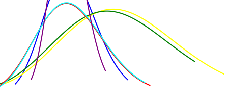
Say I would like to implement the bayesian interface in order to see the difference in the pdf of the signals. How do I approach this problem? Do I need to create multiple models and get their posterior distribution? I wanted to like visualise the change of pdf of signal 1 and signal 2 as each single will have different amplitude. Example is shown in the image

Also, side question, Can I assume that bayesian interface behaves similarly to the concept of the 1D Kalman filter where the bayesian interface can be called bayesian filter?

And what kind of step suitable for this scenario?

[Mojo_ild]

Edit 2:

If I have multiple signals can I implement it this way in order to see changes in alpha and beta in all signals?

        observed_data_S1 = pm.Beta('observed_data_S1', alpha=alpha[0], beta=beta[0], observed=S1)
        observed_data_S2 = pm.Beta('observed_data_S2', alpha=alpha[1], beta=beta[1], observed=S2)
        observed_data_S3 = pm.Beta('observed_data_S3', alpha=alpha[2], beta=beta[2], observed=S3)
        observed_data_S4 = pm.Beta('observed_data_S4', alpha=alpha[3], beta=beta[3], observed=S4)
        observed_data_S5 = pm.Beta('observed_data_S5', alpha=alpha[4], beta=beta[4], observed=S5)
        observed_data_S6 = pm.Beta('observed_data_S6', alpha=alpha[5], beta=beta[5], observed=S6)

[OriolAbril]

I noticed that you are initiating the sampler at the MAP which as explained in the FAQs, is generally not recommended. Is there any particular reason for doing so? I can’t help much with the other questions.

[Mojo_ild]

Yeah, I was following steps I found online and did not notice FAQs about the find_MAP. So, for my case I am looking at continuous distributions, so which one of the start_vals do you think I should choose for my situation?

[AlexAndorra]

Have you tried without start vals, i.e letting PyMC automatically do the work for you?
Same thing for the sampler – when you can use NUTS, use it (PyMC will automatically choose the most appropriate for you).

[Mojo_ild]

I will give it a try and return back to you

[Mojo_ild]

Well, I let it to select NUTS and removed the MAP, but, I get this error:

Auto-assigning NUTS sampler...
Initializing NUTS using jitter+adapt_diag...
Sequential sampling (3 chains in 1 job)
NUTS: [beta_S1, alpha_S1]
Sampling chain 0, 0 divergences:   0%|          | 0/2000 [00:00<?, ?it/s]
Traceback (most recent call last):
trace_S1 = pm.sample(draws=1500, tune=500, chains=3, cores=1, discard_tuned_samples=True)
trace = _sample_many(**sample_args)
**kwargs
for it, (strace, diverging) in enumerate(sampling):
for obj in iterable:
point, stats = step.step(point)
apoint, stats = self.astep(array)
raise SamplingError("Bad initial energy")
pymc3.exceptions.SamplingError: Bad initial energy

So, Where do I go from here? I know the error could be in the step, but, How can I decide what step to use?

[Mojo_ild]

Also, side question, how can I plot multiple traces in one plot? because I am looking at multiple signals and thought of combing all alphas and betas together in one plot.

[AlexAndorra]

• Bad Initial Energy can come from several issues. You can look at this entry in the FAQ.
• To plot multidimensional variables in a single plot, you can use az.plot_trace(trace, compact=True)

[Mojo_ild]

I know its a basic question, but, how can I obtain the posterior distribution of my model? and say if I used, for example, the code below from the Posterior Predictive Checks link:

_, ax = plt.subplots(figsize=(12, 6))
ax.hist([n.mean() for n in ppc['n']], bins=19, alpha=0.5)
ax.axvline(data.mean())
ax.set(title='Posterior predictive of the mean', xlabel='mean(x)', ylabel='Frequency'); 

My Code:

sns.distplot(post_pred_S1['observed_data_S1'].mean(axis=1), label='Posterior predictive means of Sensor 1 ', ax=ax)
ax.axvline(np.array(S1_ave[0]).mean(), ls='--', color='r', label='True mean of Sensor 1 ')

and found that the data mean is far away from the post pred, what do I need to do to improve the model where the mean is close to post pred?

This is how I create a model:

with pm.Model() as model_S1:
    # Prior Distributions for unknown model parameters:
    alpha_S1 = pm.HalfNormal('alpha_S1', sigma=10)
    beta_S1 = pm.HalfNormal('beta_S1', sigma=1)

    # Observed data is from a Likelihood distributions (Likelihood (sampling distribution) of observations):
    observed_data_S1 = pm.Beta('observed_data_S1', alpha=alpha_S1, beta=beta_S1,
                               observed=S1_ave)

    # instantiate sampler
    step_S1= pm.Metropolis(vars=[alpha_S1, beta_S1], model=model_S1)  ## Best one
    # step = pm.HamiltonianMC()
    # step = pm.NUTS()

    # draw 5000 posterior samples
    trace_S1 = pm.sample(draws=1500, step=step_S1, tune=500, chains=3, cores=1, discard_tuned_samples=True)

    # Obtaining Posterior Predictive Sampling:
    post_pred_S1 = pm.sample_posterior_predictive(trace_S1, samples=1000)
    print(post_pred_S1['observed_data_S1'].shape)
    print('\nSummary: ')
    print(pm.stats.summary(data=post_pred_S1))

[AlexAndorra]

The posterior samples are in trace_S1, and you can access each parameter’s posterior like in a dict: trace_S1["alpha_S1"].
Any reason why you’re using Metropolis and not letting PyMC3 choose for you? It would be NUTS in this case, which is usually recommended.

[Mojo_ild]

If you remember from previous replies, the error that I get for bad initial energy is from using NUTS (I already let the program to run with without mentioning the instantiate sampler and I get the bad initial energy), I have a question, is there a way to use MCMC as instantiate sampler?

Also, say that I use the trace samples to get the posterior samples, should I get the mean values of alpha and beta and use them to get the mean and std and use them as loc and scale of distribution to get the beta distribution shape using the scipy package or do I need to a different type of equations to calculate the lock and scale from alpha and beta to use them in the scipy package for beta distribution?
(I found this website: https://www.vosesoftware.com/riskwiki/Betadistribution.php)

[AlexAndorra]

@Mojo_ild

The error that I get for bad initial energy is from using NUTS

Bad Initial Energy usually denotes a problem with the model, not the sampler. NUTS is robust and state-of-the-art, and a good thing is that it spits out warnings when something’s wrong. Switching to an older algorithm, like Metropolis, when you don’t have to doesn’t necessarily mean the problem is gone – it’s just that the sampler doesn’t warn you about it.
So my advice would be to figure out why your model spits out a Bad Initial Energy – you’ll get a better model in the end. Here, your model uses very well-known and continuous distributions; this is NUTS kingdom

@Mojo_ild

is there a way to use MCMC as instantiate sampler?

I’m not sure I understand the question: both Metropolis and NUTS are MCMC algorithms.

@Mojo_ild

Also, say that I use the trace samples to get the posterior samples, should I get the mean values of alpha and beta

There are very good resources to introduce you to the Bayesian workflow and methods. I listed some of them here.

Hope this helps

[Mojo_ild]

Well, for my case, I have multiple lists and in the few lists, it was working fine. But, then, in one of the lists, it gives out bad initial energy. So, basically it lies within the list that I am using?

[Mojo_ild]

I managed to let the pymc3 auto assign a sampler and was using the NUTS and also managed to get some results. I have another question, if you remember my case where I have around 5 signals, I want to use for example signal 2 as my prior and signal 1 as my likelihood and posterior to be the combination of both (the concept is kind of similar to data fusion where I try to correct the data from sensor 2 with sensor 1) is this possible?

[Mojo_ild]

I have been playing with NUTS and it works fine. But, I came with problem, I was looking into the implementing for example histogram data from signals into the NUTS, however, I keep on getting the bad initial energy error. I thought at the beginning that the error is due to the outlier, so, I implement IQR outlier detection in order to remove the outliers. I removed the outliers but still I keep on getting the same error. Could it be because that there are negative values in the histogram?
Also, can you check my previous reply because I have another question?

[AlexAndorra]

I’m not sure I understand your goal and question Can you please restate them please? Ideally, can you also post the edited model, the one you say it’s working?

[Mojo_ild]

Well, Here is my new model function,

def Bayesian_Interface(data):
###################################################### Outliers ########################################################
    S_FLNO = IQR_outlier_detection(data)
    # S_FLNO = Stats_outlier_detection(data)
########################################################################################################################
    # Bayesian Model:
    with pm.Model() as model_S:
        # Prior Distributions for unknown model parameters:
        alpha_S = pm.HalfNormal('alpha_S', sigma=10)
        beta_S = pm.HalfNormal('beta_S', sigma=1)

        # Observed data is from a Likelihood distributions (Likelihood (sampling distribution) of observations):
        observed_data_S = pm.Beta('observed_data_S', alpha=alpha_S, beta=beta_S, observed=S_FLNO)

        # draw 5000 posterior samples
        trace_S = pm.sample(draws=5000, tune=2000, chains=3, cores=1)

        # Obtaining Posterior Predictive Sampling:
        post_pred_S = pm.sample_posterior_predictive(trace_S, samples=3000)
        print(post_pred_S['observed_data_S'].shape)
        print('\nSummary: ')
        print(pm.stats.summary(data=trace_S))
        print(pm.stats.summary(data=post_pred_S))
    return trace_S, post_pred_S

So, I managed to get this function to work with NUTS if I used the pdf data of the signal coming from the algorithm from link from StackOverflow (Link: https://stackoverflow.com/questions/6620471/fitting-empirical-distribution-to-theoretical-ones-with-scipy-python?noredirect=1&lq=1) [first answer], but, I keep on getting bad initial energy error again when I changed the input data into the histogram of signal or peaks of the signal. I thought because of two reasons:

• because of outliers
• because of negative values

So, I implemented the IQR outlier detection algorithm in order to detect and remove any outlier data. It managed to remove the outliers, [I used outlier detection algorithm because some data in the PDF were very high which caused bad initial energy error], but still, I keep on getting the same error. So, my question is

• Could it be, because I am using negative values into the model which also caused the bad initial energy or there could be another reason?

My second question is:

• if you remember my case where I have around 5 signals, I want to use for example signal 2 as my prior and signal 1 as my likelihood and posterior to be the combination of both (the concept is kind of similar to data fusion where I try to correct the data from sensor 2 with sensor 1) is this possible?

Side question:

What could be the reason for this warning?

The number of effective samples is smaller than 25% for some parameters.

[AlexAndorra]

Thanks, that’s much clearer.

@Mojo_ild

Could it be, because I am using negative values into the model which also caused the bad initial energy or there could be another reason?

You’re using a Beta likelihood, which has support on (0, 1), so if you’re observed values go to <= 0 or >= 1, the log probability of these points will be -inf and you’ll get bad initial energy.

So maybe the problem is that you’re not using an appropriate likelihood distribution? If your values are on the real lines, the Normal could be more appropriate – of course, this depends on your use case, domain knowledge and scientific context. If the values are too spread out, the good practice is to standardize them, otherwise the sampler is seeing a nasty geometry.

That’s probably why removing “outliers” kind of work: if you remove all the values >= 1, you don’t get -inf logp on the right hand side. But I’m very skeptical of these “outlier detections”: the risk is to end up throwing out valuable data to please the model – always better to try and adapt the model to the data instead of the opposite.

@Mojo_ild

if you remember my case where I have around 5 signals, I want to use for example signal 2 as my prior and signal 1 as my likelihood and posterior to be the combination of both (the concept is kind of similar to data fusion where I try to correct the data from sensor 2 with sensor 1) is this possible?

I’m not familiar with this concept, so I’m afraid I can’t help you here. This sounds pretty natural to express in the Bayesian framework though: just write down the prior and likelihood in your model.

@Mojo_ild

The number of effective samples is smaller than 25% for some parameters.

The sampler is having a hard time exploring the space for one or some parameters – you can usually see which with diagnostic plots and n_eff in az.summary (that’s why sampling with NUTS is a huge advantage: you get diagnostics for free).

Hope this helps

[Mojo_ild]

@AlexAndorra

I’m not familiar with this concept, so I’m afraid I can’t help you here. This sounds pretty natural to express in the Bayesian framework though: just write down the prior and likelihood in your model.

I was thinking of extracting the posterior information of say Model_S2 in order to use it as the prior in the Model_S1 and use the likelihood of observed_data_S1. Am I going the right way? If it is, how can I extract the posterior information from Model_S2