How to implement Hierarchical Gaussian Process in PyMC?

[TPK]

Hello, I’m not sure if this topic had been answered or not, and I’m not familiar with Gaussian Process.
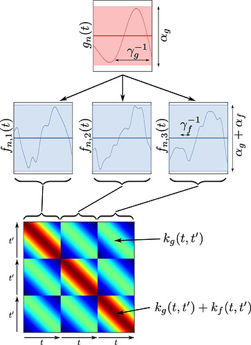
But I am trying to implement Hierarchical Gaussian Process (HGP) based on Hensman, et al (2013). This implementation is implemented in GPy package, and the example notebook can be found here

The idea from the paper is this

which can be extended further as

The paper illustrate the model as

where

But as of right now, I don’t really understand PyMC gaussian process enough to implement this. Any guidance is welcome

Thanks!

---

This is my attempt of following this example, but I think this is still incorrect, and it sample really slow too

Setup + Generate Data

import arviz as az
import matplotlib.pyplot as plt
import numpy as np
import pymc as pm

%config InlineBackend.figure_format = 'retina'
RANDOM_SEED = 8998
rng = np.random.default_rng(RANDOM_SEED)
az.style.use("arviz-darkgrid")

n_grps = 3
n = 20  # The number of data points
X = np.linspace(0, 10, n_grps * n)[:, None]  # The inputs to the GP must be arranged as a column vector

# Define the true covariance function and its parameters
ell_true = 1.0
eta_true = 4.0
cov_func = eta_true**2 * pm.gp.cov.ExpQuad(1, ell_true)

# A mean function that is zero everywhere
mean_func = pm.gp.mean.Zero()

# The latent function values are one sample from a multivariate normal
# Note that we have to call `eval()` because PyMC built on top of Theano
f_true = pm.draw(pm.MvNormal.dist(mu=mean_func(X), cov=cov_func(X)), 1, random_seed=rng)

# The observed data is the latent function plus a small amount of T distributed noise
# The standard deviation of the noise is `sigma`, and the degrees of freedom is `nu`
sigma_true = 1.0
nu_true = 5.0
y = f_true + sigma_true * rng.normal(size=n_grps * n)

indices = np.sort(np.random.permutation(len(y)).reshape(n_grps, n))
X_i = X.reshape(-1)[indices].reshape(n_grps, n, 1)
y_i = y[indices]

## Plot the data and the unobserved latent function
fig = plt.figure(figsize=(10, 4))
ax = fig.gca()
ax.plot(X, f_true, "dodgerblue", lw=3, label="True generating function 'f'")
# ax.plot(X, y, "ok", ms=3, label="Observed data")
for i in range(n_grps):
    ax.plot(X_i[i], y_i[i], "o", lw=2, label=f"Partial Obs [{i + 1}]")
ax.set_xlabel("X")
ax.set_ylabel("y")
plt.legend(frameon=True);

Attempt #1

with pm.Model() as model:
    ell = pm.Gamma("ell", alpha=2, beta=1)
    eta = pm.HalfNormal("eta", sigma=5)

    cov_1 = eta**2 * pm.gp.cov.ExpQuad(1, ell)
    gp_1 = pm.gp.Latent(cov_func=cov_1)
    
    f_i = [gp_1.prior(f"f_{i}", X=X_i[i]) for i in range(n_grps)]
    
    ell_2 = pm.Gamma("ell_2", alpha=2, beta=1, shape=(n_grps,))
    eta_2 = pm.HalfNormal("eta_2", sigma=5, shape=(n_grps,))
    conv_2s = [eta_2[i]**2 * pm.gp.cov.ExpQuad(1, ell_2[i]) for i in range(n_grps)]
    gp_2s = [pm.gp.Latent(cov_func=conv_2s[i]) for i in range(n_grps)]
    
    g_i = [gp_2s[i].prior(f"g_{i}", X=f_i[i].reshape((X_i.shape[1], 1))) for i in range(n_grps)]

    sigma = pm.HalfNormal("sigma", sigma=2.0, shape=(n_grps,))
    nu = 1 + pm.Gamma(
        "nu", alpha=2, beta=0.1, shape=(n_grps,)
    )  # add one because student t is undefined for degrees of freedom less than one
    y_ = [pm.StudentT(f"y_{i}", mu=g_i[i], lam=(1.0/sigma[i]), nu=nu[i], observed=y_i[i]) for i in range(n_grps)]

    idata = pm.sample(200, tune=200, chains=2, cores=6)

Plot

f_posts = az.extract(idata, var_names=[f"f_{i}" for i in range(n_grps)]).transpose("sample", ...)
g_posts = az.extract(idata, var_names=[f"g_{i}" for i in range(n_grps)]).transpose("sample", ...)

# plot the results
fig = plt.figure(figsize=(10, 4))
ax = fig.gca()

color_palette = ["Reds", "Greens", "Blues"]
# for i in range(n_grps):
#     plot_gp_dist(ax, f_posts[f"f_{i}"], X_i[i], palette=color_palette[i])
for i in range(n_grps):
    plot_gp_dist(ax, g_posts[f"g_{i}"], X_i[i], palette=color_palette[i])

# plot the data and the true latent function
ax.plot(X, f_true, "dodgerblue", lw=3, label="True generating function 'f'")
ax.plot(X, y, "ok", ms=3, label="Observed data")

# axis labels and title
plt.xlabel("X")
plt.ylabel("True f(x)")
plt.title("Posterior distribution over $f(x)$ at the observed values")
plt.legend();

---

Attempt #2

This version is worse

with pm.Model() as model:
    ell = pm.Gamma("ell", alpha=2, beta=1)
    eta = pm.HalfNormal("eta", sigma=5)

    cov_1 = eta**2 * pm.gp.cov.ExpQuad(1, ell)
    gp_1 = pm.gp.Latent(cov_func=cov_1)
    
    f = gp_1.prior("f", X=X_i.reshape(-1, 1))
    f_reshape = f.reshape(X_i.shape)
    
    ell_2 = pm.Gamma("ell_2", alpha=2, beta=1, shape=(n_grps,))
    eta_2 = pm.HalfNormal("eta_2", sigma=5, shape=(n_grps,))
    conv_2s = [eta_2[i]**2 * pm.gp.cov.ExpQuad(1, ell_2[i]) for i in range(n_grps)]
    gp_2s = [pm.gp.Latent(cov_func=conv_2s[i]) for i in range(n_grps)]
    
    g_i = [gp_2s[i].prior(f"g_{i}", X=f_reshape[i].reshape((X_i.shape[1], 1))) for i in range(n_grps)]

    sigma = pm.HalfNormal("sigma", sigma=2.0, shape=(n_grps,))
    nu = 1 + pm.Gamma(
        "nu", alpha=2, beta=0.1, shape=(n_grps,)
    )  # add one because student t is undefined for degrees of freedom less than one
    y_ = [pm.StudentT(f"y_{i}", mu=g_i[i], lam=(1.0/sigma[i]), nu=nu[i], observed=y_i[i]) for i in range(n_grps)]

    idata = pm.sample(400, tune=400, chains=2, cores=6)

[TPK]

I think I’m getting closer. What I ended up doing is porting the code from GPy. But I have absolutely no confidence that this is correct. Still the result did look nice

A bit of context. The input X must include grouping columns (indicate by extra_dims). So the entire input space need to be concatenate together to form X input. Now, I only tested for 2 levels, but 3 levels should be fine (I think)

Also the sampling performance might be hit-or-miss. I tried increase n_grps = 4. The NUTS sampling rate slowed down from ~3 minutes to over 2-3 hours. I’m not sure what is happening here

If anyone is familiar with HGP, please check my work

Setup Code

%config InlineBackend.figure_format = 'retina'
import GPy
import pymc as pm
import arviz as az
import numpy as np
import pytensor.tensor as pt
import matplotlib.pyplot as plt
from pymc.gp.util import plot_gp_dist

az.style.use("arviz-darkgrid")

np.random.seed(1337)
n_grps = 3
colors = ["lightcoral", "firebrick", "maroon"] 
T = np.linspace(0, 20, 300).reshape(-1, 1)

#construce kernel (covariance function) objects
kern_upper = GPy.kern.Matern32(input_dim=1, variance=1.0, lengthscale=3.0)
kern_lower = GPy.kern.Matern32(input_dim=1, variance=0.25, lengthscale=5.0)

#compute the covariance matrices
K_upper = kern_upper.K(T)
K_lower = kern_lower.K(T)

g = np.random.multivariate_normal(np.zeros(len(T)), K_upper)
f = []
for r in range(n_grps):
    f.append(np.random.multivariate_normal(g, K_lower))

max_samples = np.clip(np.random.uniform(0, 0.2*len(T), size=n_grps).astype(np.int32), 1, len(T))
selected_indices = [np.sort(np.random.permutation(len(T))[:max_samples[i]]) for i in range(n_grps)]

X_i = [T[selected_indices[i]] for i in range(n_grps)]
y_i = [f[i][selected_indices[i]] for i in range(n_grps)]

plt.plot(T, g, color="k")
for i in range(n_grps):
    plt.plot(T, f[i], "--", color=colors[i])
    plt.plot(X_i[i], y_i[i], "o", color=colors[i])
plt.show()

X, y = [], []
for i in range(len(X_i)):
    X.append(np.concatenate([X_i[i], i*np.ones_like(X_i[i])], axis=-1))
X = np.concatenate(X)
y = np.concatenate(y_i)

Custom Covariance

def index_to_slices(index):
    # From https://github.com/SheffieldML/GPy/blob/devel/GPy/util/multioutput.py
    if len(index)==0:
        return[]

    #contruct the return structure
    ind = np.asarray(index,dtype=np.int)
    ret = [[] for i in range(ind.max()+1)]

    #find the switchpoints
    ind_ = np.hstack((ind,ind[0]+ind[-1]+1))
    switchpoints = np.nonzero(ind_ - np.roll(ind_,+1))[0]

    [ret[ind_i].append(slice(*indexes_i)) for ind_i,indexes_i in zip(ind[switchpoints[:-1]],zip(switchpoints,switchpoints[1:]))]
    return ret

class Hierarchical(pm.gp.cov.Covariance):
    # Not sure if this should be `pm.gp.cov.Combination`
    def __init__(self, kernels):
        assert len(kernels) >= 2
        assert all([k.input_dim == kernels[0].input_dim for k in kernels])
        assert all([all(k.active_dims == kernels[0].active_dims) for k in kernels])
        input_max = max([k.input_dim for k in kernels])
        
        super().__init__(
            input_dim=kernels[0].input_dim,
            active_dims=kernels[0].active_dims
        )
        self.kernels = kernels
        self.extra_dims = range(input_max, input_max + len(kernels)-1)
    
    def call_kern(self, kernel, X, Xs):
        if isinstance(kernel, pm.gp.cov.Combination):
            return kernel(X, Xs)
        return kernel.full(X, Xs)
    
    def full(self, X, Xs=None):
        # Base kernel
        kernel = self.call_kern(self.kernels[0], X, Xs)
        
        X_slices = [
            index_to_slices(X[:, i]) for i in self.extra_dims
        ]
        
        if Xs is None:
            for k, slices_k in zip(self.kernels[1:], X_slices):
                for slices_i in slices_k:
                    for s in slices_i:
                        kernel = pt.set_subtensor(kernel[s, s], kernel[s, s] + self.call_kern(k, X[s], None))
        else:
            Xs_slices = [
                index_to_slices(Xs[:,i]) for i in self.extra_dims
            ]
            for k, slices_k1, slices_k2 in zip(self.kernels[1:], X_slices, Xs_slices):
                for slices_i, slices_j in zip(slices_k1, slices_k2):
                    for s, ss in zip(slices_i, slices_j):
                        kernel = pt.set_subtensor(kernel[s, ss], kernel[s, ss] + self.call_kern(k, X[s], Xs[ss]))
        return kernel
    
    def diag(self, X):
        return pt.diag(self.full(X, None))

Modeling

with pm.Model() as model:
    # Upper Covariance
    upper_ell = pm.Gamma("upper_ell", alpha=2, beta=1)
    upper_eta = pm.HalfNormal("upper_eta", sigma=5)
    upper_cov = upper_eta**2 * pm.gp.cov.ExpQuad(1, upper_ell, active_dims=[0])
    
    # Lower Covariance
    lower_ell = pm.Gamma("lower_ell", alpha=2, beta=1)
    lower_eta = pm.HalfNormal("lower_eta", sigma=5)
    lower_cov = lower_eta**2 * pm.gp.cov.ExpQuad(1, lower_ell, active_dims=[0])
    
    # Combined Covariance
    h_cov = Hierarchical([upper_cov, lower_cov])
    gp = pm.gp.Latent(cov_func=h_cov)
    
    f = gp.prior("f", X=X)
    sigma = pm.HalfNormal("sigma", sigma=2.0)
    nu = 1 + pm.Gamma(
        "nu", alpha=2, beta=0.1
    )  # add one because student t is undefined for degrees of freedom less than one
    y_ = pm.StudentT(f"y", mu=f, lam=(1.0/sigma), nu=nu, observed=y)

    idata = pm.sample(100, tune=100, chains=2, cores=6)

    # Predictions
    f_preds = [gp.conditional(f"f_preds_{i}", np.concatenate([T, i * np.ones_like(T)], axis=1), jitter=1e-4) for i in range(n_grps)]
    ppc = pm.sample_posterior_predictive(
        idata.posterior, var_names=sum([[f"f_preds_{i}"] for i in range(n_grps)], [])
    )

Ploting

f_posts = az.extract(ppc.posterior_predictive, var_names=[f"f_preds_{i}" for i in range(n_grps)]).transpose("sample", ...)

fig = plt.figure(figsize=(10, 4))
ax = fig.gca()

color_palette = ["Reds", "Greens", "Blues"]
for i in range(n_grps):
    plot_gp_dist(ax, f_posts[f"f_preds_{i}"], T, palette=color_palette[i], samples_alpha=0.5)

# axis labels and title
plt.xlabel("X")
plt.ylabel("True f(x)")
plt.title("Posterior distribution over $f(x)$ at the observed values")
plt.show()

fig, axes = plt.subplots(n_grps + 1, 1, figsize=(10, 4*(n_grps + 1)), sharex=True)
color_palette = ["Reds", "Greens", "Blues"]
colors = ["red", "green", "blue"]
axes[0].plot(T, g, color="k", label="True Upper")
for i in range(n_grps):
    axes[0].plot(T, f_true[i], "-", color=colors[i], label=f"True Lower[{i}]")
    axes[0].plot(
        T_new[(T_new >= T.min()) & (T_new <= T.max())],
        f_posts[f"f_preds_{i}"].mean(["sample"]).to_numpy()[((T_new >= T.min()) & (T_new <= T.max())).reshape(-1)],
        "--", color=colors[i], alpha=0.5
    )
    axes[0].legend(loc="best")
    plot_gp_dist(axes[i + 1], f_posts[f"f_preds_{i}"], T_new, palette=color_palette[i])
    axes[i + 1].plot(T, f_true[i], color="dodgerblue", label="True Lower")
    axes[i + 1].plot(X_i[i], y_i[i], "ok", label="Samples")
    axes[i + 1].legend(loc="best")

plt.suptitle("Diagnosis Plot")
plt.show()

[bwengals]

See Improve NUT sampling rate in Gaussian Process when using custom Covariance - #2 by bwengals, which I meant to post here

[TPK]

I am able to apply your code to my example (variable length + larger group). It is a bit janky but work

sorted_indice = np.argsort(X[:, 0])
sorted_X = X[sorted_indice][:, 0].reshape(-1, 1)
groups_X = X[sorted_indice][:, 1].astype(np.int32)
sorted_y = y[sorted_indice]
grp_idxes = np.unique(groups_X)

partition_idxes = {
    k: np.arange(sorted_X.shape[0])[groups_X == k] for k in grp_idxes
}
partition_y = { k: sorted_y[partition_idxes[k]] for k in partition_idxes.keys() }

with pm.Model() as model:
    X_ = pm.MutableData("X", sorted_X)
    grp_ = pm.MutableData("grp", groups_X)
    y_ = pm.MutableData("y", sorted_y)
    
    lower, upper = 0.5, 3
    ell_g_params = pm.find_constrained_prior(
        pm.InverseGamma,
        lower, upper, 
        init_guess={"alpha": 2, "beta": 20},
        mass=0.95
    )
    ell_g = pm.InverseGamma("ell_g", **ell_g_params)
    est_scale = 2.0
    eta_g = pm.Exponential("eta_g", lam = 1.0 / est_scale)
    cov_g = eta_g**2 * pm.gp.cov.ExpQuad(input_dim=1, ls=ell_g)
    gp_g = pm.gp.HSGP(m=[200], c=1.5, cov_func=cov_g)
    g = gp_g.prior("g", X=X_)
    
    lower, upper = 0.5, 3
    ell_f_params = pm.find_constrained_prior(
        pm.InverseGamma,
        lower, upper, 
        init_guess={"alpha": 2, "beta": 20},
        mass=0.95
    )
    ell_f = pm.InverseGamma("ell_f", **ell_f_params)
    eta_f = pm.Exponential("eta_f", lam = 1.0 / est_scale)
    cov_f = eta_f**2 * pm.gp.cov.ExpQuad(input_dim=1, ls=ell_f)
    
    sigma = pm.Exponential("sigma", lam=1.0/2.0)
    nu = pm.Gamma("nu", alpha=2, beta=1)
    
    gp_fs = []
    for i in sorted(grp_idxes):
        mask = pt.arange(X_.shape[0])[pt.abs(grp_ - i) <= 1e-3]
        gp_f = pm.gp.HSGP(m=[200], c=1.5, cov_func=cov_f)
        gp_fs.append(gp_f)
        delta = gp_f.prior(f"delta_{i}", X=X_[mask])
        replicate = pm.Deterministic(f"f_{i}", g[mask] + delta)
        pm.StudentT(
            f"lik_{i}",
            mu=replicate,
            sigma=sigma, nu=nu,
            observed=partition_y[i]
        )

### Prediction
mag = (T.max() - T.min())
new_mag = 2*mag

centre = (T.min() + T.max())/2
grp_idxes = [*list(range(n_grps))]
T_new = np.linspace(centre - new_mag//2, centre + new_mag//2, 100).reshape(-1, 1)
T_new_cats = [np.concatenate([T_new, i * np.ones_like(T_new)], axis=1) for i in grp_idxes]

with model:
    idata = pm.sample(
        nuts_sampler="numpyro",
        draws=1000,
        tune=1000,
        chains=2,
        cores=4,
        random_seed=rng
    )
    
    g_preds = gp_g.conditional("g_pred", T_new.reshape(-1, 1))
    fpreds = [gp_fs[i].conditional(f"f_preds_{i}", T_new_cats[i]) for i in range(len(gp_fs))]
    ppc = pm.sample_posterior_predictive( 
        idata.posterior, var_names=sum([[f"f_preds_{i}"] for i in grp_idxes], ["g_pred"]),
        random_seed=rng
    )

### Plots
fig = plt.figure(figsize=(15, 7))
gs = fig.add_gridspec(nrows=3, ncols=5, height_ratios=[2, 0.5, 0.5])

ax = fig.add_subplot(gs[0, :])
g_pred = ppc.posterior_predictive["g_pred"].stack(sample=["chain", "draw"])

lower = np.percentile(g_pred.data, 5,  axis=1)
upper = np.percentile(g_pred.data, 95, axis=1)
mean = np.mean(g_pred.data, axis=1)
ax.scatter(X[:, 0], y, c="k", s=14, zorder=2)
ax.plot(T_new.reshape(-1), mean, color="k")
ax.fill_between(T_new.reshape(-1), lower, upper, color="k", alpha=0.4);

for i in grp_idxes:
    color = "C" + str(i)
    f_pred = ppc.posterior_predictive[f"f_preds_{i}"].stack(sample=["chain", "draw"])
    pred = (f_pred.to_numpy() + g_pred.to_numpy())
    lower = np.percentile(pred, 5,  axis=1)
    upper = np.percentile(pred, 95, axis=1)
    mean = np.mean(pred, axis=1)
    
    ax = fig.add_subplot(gs[int(i//5) + 1, i%5])
    ax.plot(T_new.reshape(-1), mean, color=color)
    ax.fill_between(T_new.reshape(-1), lower, upper, color=color, alpha=0.4);
    ax.scatter(X[X[:, 1] == i][:, 0], y[X[:, 1] == i], c="k", s=5, zorder=2)
    ax.xaxis.set_tick_params(labelbottom=False)
    ax.yaxis.set_tick_params(labelleft=False)
plt.show()

[bwengals]

Looks nice! Since you’re going from -40 to 40, you may need to use a larger c value. It basically controls the domain the approximation is accurate. With c=1.5, and your data ranging from -20 to 20, c=1.5 means that your approximation is accurate from -30 to 30. (which is c times half range of data = means from -30 to 30). You can see the little dip there at -30 and 30. If you plot a higher resolution, you’ll see it go to zero there and get wonky beyond that.