How to mix known and unkwon information for Covariance Matrix?

[Mister-Knister]

Hey,
I have a data matrix Y (NxK) and a matrix for the errors: E (NxK).

I now assume the following model:

Y_{i,j} = a_i + b_j +u_{i,j} with u_{i,j} \sim N(0, e_{i,j}^2 + d_j^2 + g_i^2).

I want to fit the model to find the parameters a, b, d and g. I have already set up a test model for the regression for a and b. For simplicity I assumed that the errors are equal to 1.

import numpy as np
import pymc3 as pm
import theano
import theano.tensor as tt
np.random.seed(123456)

#set dimension of data matrix
dim_N = 5  
dim_K = 20

#create test data
a = np.random.normal(1.5, 10, dim_N)
b = np.random.normal(-1, 1, dim_K)
y = a[:, np.newaxis] + b

#create design matrices alpha and beta such that: 
#y_vec = alpha @ [a_1, a_2 ..., a_N] + beta @ [b_1, b_2, ..., b_K]

alpha = np.zeros(shape=(dim_N * dim_K, dim_N), dtype= theano.config.floatX)
beta = np.zeros(shape=(dim_N * dim_K, dim_K), dtype= theano.config.floatX)

for i in range(0, dim_N*dim_K):
    for j in range(0, dim_N):
        if ((i % (dim_N)) == j):
            alpha[i, j] = 1
            
for i in range(0, dim_N*dim_K):
    for j in range(0, dim_K):
        if ((np.floor(i/dim_N)) == j):
            beta[i, j] = 1
#flatten the data matrix, so that it can be described by pm.Normal or pm.MvNormal
y_vec = y.flatten("F")


model = pm.Model()
with model:
    #priors on a and b
    a = pm.Normal("a", mu = 0, sigma = 15, shape = dim_N)
    b = pm.Normal("b", mu = 0, sigma = 1, shape = dim_K)
    #calculate mu = alpha @ a + beta @ b
    mu = tt.nlinalg.matrix_dot(alpha, a) + tt.nlinalg.matrix_dot(beta, b)
    #define likelihood
    likelihood = pm.Normal("y", mu = mu, sd=1, observed=y_vec)

#sample
with model:
    trace = pm.sample(5000, cores=4, chains=4, tune=10000)

My model breaks down however when I want to include the error matrix and the regression on the unknown variance parameters d and g. Especially if I want to also regress on potential correlations. Here I would need to use LKJcholeskyCov, but again I am not sure how to combine known and unknown information . I am very thankful for any hint!

[chartl]

Hi Mister-Knister,

It looks like you’re fitting a linear mixed model.

A nice rule of thumb that works for me for pymc3 is to start by writing a model to simulate data – I often find that an observed= can be placed in an obvious place. In this case we’d have

import pymc3 as pm
import theano
import theano.tensor as tt
import numpy as np
import seaborn as sbn
from matplotlib import pyplot as plt

n_treatments = 8
n_groups = 12

print('Total DOF: {}  Used DOF: {}  Remaining DOF: {}'.format(
    n_treatments*n_groups, 2*n_treatments + 2*n_groups + 1, 
    n_treatments*n_groups - (2*n_treatments + 2*n_groups + 1)
    ))

var_treat_ = 1 + np.arange(n_treatments, dtype=np.float32)/n_treatments
var_group_ = 1 + np.arange(n_groups, dtype=np.float32)

mean_treat_ = -np.arange(n_treatments, dtype=np.float32)
mean_groups_ = -np.arange(n_groups, dtype=np.float32)

with pm.Model() as model_univar:
    mu_t_noise = pm.Normal('_mu_t_noise', 0, 1e-3, shape=n_treatments)
    mean_treat = (mu_t_noise + mean_treat_).reshape((n_treatments, 1))
    mu_g_noise = pm.Normal('_mu_g_noise', 0, 1e-3, shape=n_groups)
    mean_group = (mu_g_noise + mean_groups_).reshape((1, n_groups))
    log_sd_t_noise = pm.Normal('_t_noise', 0, 1e-3, shape=n_treatments)
    log_sd_g_noise = pm.Normal('_g_noise', 0, 1e-3, shape=n_groups)
    sd_treat = tt.exp(log_sd_t_noise + 0.5 * np.log(var_treat_)).reshape((n_treatments, 1))
    sd_group = tt.exp(log_sd_g_noise + 0.5 * np.log(var_group_)).reshape((1, n_groups))
    sd_noise = 1e-4
    
    mean_mat = mean_treat + mean_group
    sd_mat = sd_treat + sd_group + sd_noise
    
    Y_obs = pm.Normal('Y_obs', mu=mean_mat, sd=sd_mat, shape=(n_treatments,n_groups))
    
    trace = pm.sample_prior_predictive(10)
    sbn.heatmap(trace['Y_obs'][0,:,:]);

Total DOF: 96 Used DOF: 41 Remaining DOF: 55

def noncentered_param(basename, shape=None, reshape=None):
    names = {'sd': '{}_sd'.format(basename),
             'offset': '{}_offset'.format(basename),
             'mu': '{}_mu'.format(basename)}
    sd = pm.HalfNormal(names['sd'], 1, shape=shape)
    mu = pm.Normal(names['mu'], 0, 1, shape=shape)
    off = pm.Normal(names['offset'], 0, 1, shape=shape)
    var = pm.Deterministic(basename, mu + sd * off)
    if reshape:
        return var.reshape(reshape)
    return var


with pm.Model() as model_univar_inf:
    mean_treat = noncentered_param('mean_treat', n_treatments, (n_treatments,1))
    mean_group = noncentered_param('mean_group', n_groups, (1, n_groups))
    sd_treat = tt.exp(noncentered_param('sd_treat_log', n_treatments, (n_treatments,1)))
    sd_group = tt.exp(noncentered_param('sd_group_log', n_groups, (1, n_groups)))
    sd_noise = pm.HalfNormal('sd_err', 1.)
    
    mean_mat = mean_treat + mean_group
    sd_mat = sd_treat + sd_group + sd_noise
    
    Y_obs = pm.Normal('Y_obs', mu=mean_mat, sd=sd_mat, shape=(n_treatments,n_groups), observed=trace['Y_obs'][0,:,:])
    
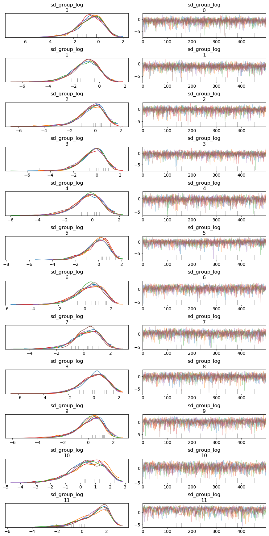
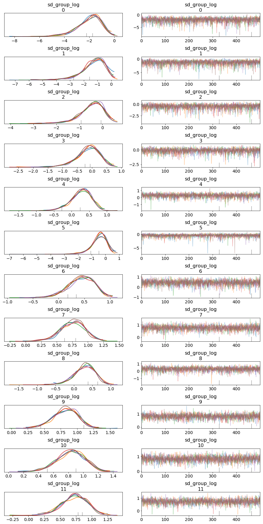
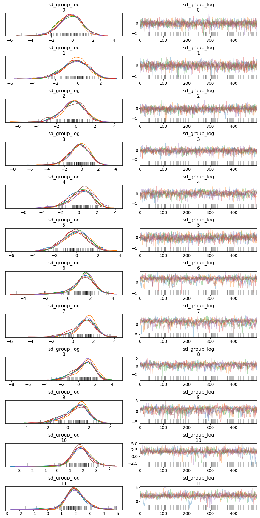
    inf_trace = pm.sample(500, tune=1000, chains=6)

pm.traceplot(inf_trace, ['sd_group_log']);

You can also have multiple observations along the 0th axis (though this is not likely to be your use case)

    Y_obs = pm.Normal('Y_obs', mu=mean_mat, sd=sd_mat, shape=(n_treatments,n_groups), observed=trace['Y_obs'][:,:,:])
    
    inf_trace = pm.sample(500, tune=1000, chains=6)

When moving to correlations, the typical way is to note that the model above (where sd_mat is explicit) is equivalent (for a single matrix observation) to this model:

with pm.Model() as model_latent_var:
    mean_treat = noncentered_param('mean_treat', n_treatments, (n_treatments,1))
    mean_group = noncentered_param('mean_group', n_groups, (1, n_groups))
    # note that reshaping no longer happens here
    sd_treat = tt.exp(noncentered_param('sd_treat_log', n_treatments))
    sd_group = tt.exp(noncentered_param('sd_group_log', n_groups))
    sd_noise = pm.HalfNormal('sd_err', 1.)
    
    z_treat = pm.Deterministic('z_treat', pm.Normal('_z_treat_offset', 0, 1, shape=n_treatments) * sd_treat).reshape((n_treatments,1))
    z_group = pm.Deterministic('z_group', pm.Normal('_z_group_offset', 0, 1, shape=n_groups) * sd_group).reshape((1, n_groups))
    
    mean_mat = (mean_treat + mean_group) + (z_treat + z_group)
    
    Y_obs = pm.Normal('Y_obs', mu=mean_mat, sd=sd_noise, shape=(n_treatments,n_groups), observed=trace['Y_obs'][0,:,:])
    
    inf_trace = pm.sample(500, tune=1000, chains=6)

it is slower (and harder) to sample, as the sampler needs to marginalize over the new z variables; but it gives you more direct control over defining (marginal) correlations between treatments and groups (rows and columns); by allowing you to make more complicated models for z.

If you can define the marginal relationships (row covariance, column covariance) explicitly, take a look at pm.MatrixNormal.

Note, especially, that the “full” covariance for a (N,K) matrix is in fact an (N, K, N, K) tensor because of terms like \mathrm{cor}(X_{1,3},X_{2,8}). In the rare case where you want to test particular structures for that tensor, you still need to unwrap the (N,K) matrix into an (NK, 1) vector, and specify the tensor as the appropriate (NK,NK) matrix.

[Mister-Knister]

Hey Chartl,

thank you very much for your very instructive post! I will keep in mind to use simulations in the future. If you don’t mind, I have 5 follow up questions regarding your post and for my better understanding of pymc3:

regarding your post:

1.) why do you use the log of the standard error? Is it numerically more stable?
2.) I don’t understand what you did with the z_treat and z_group. I think I lack the theoretical knowledge here. Any hint in which direction I should look into?

regarding PYMC3:

4.) when should I use pm.Deterministic? Still can’t quite get my head around that. What would happen if you would have omitted it?
3.) just for completeness, in my code example I used design matrices to construct my mu vector. I did it in this way because I didn’t know if that would have been possible with loops. Can I fill an array(tensor) with stochastic variables, maybe even from different distributions, i.e.: mu = [pm.Uniform(0, 2), pm.Normal(0, 10)…]. Do I need theano.scan for this?
5.) Can I use LKJcholeskyCov to estimate the offdiagonal elements of the covariance matrix ((NK, NK) tensor)? LKJcholeskyCov takes a distribution for the standard error. Can I define a custom distribution where sd is an 1D array with each entry defined by the model (vec( e_{ij}^2 + d_j^2 + g_i^2))?

Cheers,
Mister-Knister

[chartl]

1. I’m using a non-centered parametrization of a log-normal prior. The prior you choose is up to you.
2. The z_treat and z_group is a parameterization trick commonly used in mixed-effects models. These are typically marginalized out to get a likelihood; but you can perform that marginalization numerically (as is done here).
3. You can use set_subtensor or even tt.stack with a list.
4. pm.Deterministic just registers a theano variable with the model, so that its sampled values will be available in a trace. If you don’t include it, then the values will be simulated, but not tracked.
5. (a) Theoretically you can use LKJCholeskyCov to do this; but I doubt you have the >N^2K^2 observations required for the model to be well-specified. You could borrow from the Factor Analysis example and use a diagonal-plus-low-rank approximation.
6. (b) [this is a 5) in the source of the post ] There’s no need to define a custom distribution for this. In fact, you would just get this from

pm.Normal('obs',
   mu=mean_mat.reshape((N*K,)),
   sd=sd_mat.reshape((N*K,)),
   observed=Y.reshape((N*K,)))