Implementing rounding (by manual integration) more efficiently

I would like to use the following distribution as a part of my model

import pymc as pm
from pymc.math import log, exp

def _podium_logp(value, mu, sigma):
    dist = pm.Gamma.dist(mu=mu, sigma=sigma)

    density1 = exp(pm.logcdf(dist, value + 3)) - exp(pm.logcdf(dist, value - 2))
    density2 = exp(pm.logcdf(dist, value + 2)) - exp(pm.logcdf(dist, value - 1))
    density3 = exp(pm.logcdf(dist, value + 1)) - exp(pm.logcdf(dist, value))

    return log(5 / 9 * density1 + 3 / 9 * density2 + 1 / 9 * density3)

pm.CustomDist("y", mu, sigma, logp=_podium_logp)

Are there any obvious ways I could make a faster implementation? The current one seems to work but it would be way more usable if it was faster.

I tested the speed of my current implementation by using both the default for pm.sample’s option nuts_sampler and blackjax. With the default sampler, I was unable to get any results as it took minutes to get a single sample during tuning. With blackjax, the implementation was roughly 60 times slower than just using a Gamma distribution and roughly 2.7 times slower than using PyTensor’s floor function or manually calculating the rounding likelihood.

I’ll post a more detailed explanation, some motivation and some of my test results in the replies. Feel free to skip it. It’s honestly a bit convoluted and maybe not that important.

I’m using pymc==5.10.3 and blackjax==1.0.0 on a Windows machine if that matters.

A longer explanation:

I’m making a model for intervals between events. The data (timestamps of the events) for my model were collected with the timestamps having a resolution of one second (rounded down). The way these timestamps were collected wasn’t the most accurate, but I’m fairly certain that they’re usually off by one second at most. Hence I have a discrete uniform error distribution with support {-1,0,1} for the timestamps plus a maximum of one second of rounding error.

Since I’m modelling the intervals, the error distribution ends up being (after assuming independent errors for the timestamps and doing some simple combinatorics)

p(x) = \begin{cases} 1/9, &-2 \leq x < -1\\ 2/9, &-1 \leq x < 0\\ 3/9, &0 \leq x < 1\\ 2/9, &1 \leq x < 2\\ 1/9, &2 \leq x < 3\\ \end{cases}
I called this “podium” in the code since its shape resembles the shape of a winners’ podium. This might not be the “true” error distribution but the inference results seem to be somewhat unstable w.r.t. the choice of error distribution and I’d like to also see the results from this one.

For the underlying distribution of the unrounded intervals, I used Gamma. This also might not be the final choice but it felt like an OK first guess. It also has a nice feature of highlighting the issues with using the wrong error distribution in the model. I’m using mean/variance parametrization and the mean is estimated well from simulated data by just taking the rounding into account. The variance however need an correctly defined error distribution.

I felt that the most straightforward way for me to implement this error distribution with pymc was by constructing it as a mixture three different components as seen in the first post. I also tried the perhaps more readable way of using pm.Mixture but it wasn’t any faster.

I made the following toy example for testing the model

import numpy as np
import pymc as pm
from pymc.math import floor, log, exp
import pytensor.tensor as pt
import arviz
from pandas import DataFrame


def _create_data(data_count):

    model = pm.Model()
    with model:
        raw = pm.Gamma(
            "raw", mu=11, sigma=2  # mu set high and sigma low to avoid values < 3
        )
        rounded = pm.Deterministic("rounded", floor(raw))

        uniform_error = pm.DiscreteUniform("uniform_error", lower=-1, upper=1)
        pm.Deterministic("uniform", rounded + uniform_error)

        podium_error = pm.Mixture(
            "podium_error",
            [5 / 9, 3 / 9, 1 / 9],
            [
                pm.DiscreteUniform.dist(-2, 2),
                pm.DiscreteUniform.dist(-1, 1),
                pm.DiscreteUniform.dist(0, 0),
            ],
        )
        pm.Deterministic("podium", rounded + podium_error)

        data = pm.sample_prior_predictive(samples=data_count, random_seed=1).prior

    return (
        data.raw.values.flatten(),
        data.rounded.values.flatten(),
        data.uniform.values.flatten(),
        data.podium.values.flatten(),
    )


def _floor_dist(mu, sigma, size):
    raw_dist = pm.Gamma.dist(mu=mu, sigma=sigma, size=size)
    return pt.floor(raw_dist)


def _flexible_floor_logp(value, mu, sigma, lower, upper):
    dist = pm.Gamma.dist(mu=mu, sigma=sigma)

    density = exp(pm.logcdf(dist, value + upper)) - exp(pm.logcdf(dist, value + lower))

    return log(density)


def _podium_logp(value, mu, sigma):
    dist = pm.Gamma.dist(mu=mu, sigma=sigma)

    density1 = exp(pm.logcdf(dist, value + 3)) - exp(pm.logcdf(dist, value - 2))
    density2 = exp(pm.logcdf(dist, value + 2)) - exp(pm.logcdf(dist, value - 1))
    density3 = exp(pm.logcdf(dist, value + 1)) - exp(pm.logcdf(dist, value))

    return log(5 / 9 * density1 + 3 / 9 * density2 + 1 / 9 * density3)


def _create_models(data):
    naive_model = pm.Model()
    with naive_model:
        mu = pm.Normal("mu", mu=0, sigma=10)
        sigma = pm.HalfNormal("sigma", sigma=10)

        mutable_data = pm.MutableData("data", data)
        pm.Gamma("y", mu=mu, sigma=sigma, observed=mutable_data)

    rounded_model = pm.Model()
    with rounded_model:
        mu = pm.Normal("mu", mu=0, sigma=10)
        sigma = pm.HalfNormal("sigma", sigma=10)

        mutable_data = pm.MutableData("data", data)
        pm.CustomDist(
            "y",
            mu,
            sigma,
            dist=_floor_dist,
            observed=mutable_data,
        )

    uniform_model = pm.Model()
    with uniform_model:
        mu = pm.Normal("mu", mu=0, sigma=10)
        sigma = pm.HalfNormal("sigma", sigma=10)

        mutable_data = pm.MutableData("data", data)
        pm.CustomDist(
            "y",
            mu,
            sigma,
            -1,
            2,
            logp=_flexible_floor_logp,
            observed=mutable_data,
        )

    podium_model = pm.Model()
    with podium_model:
        mu = pm.Normal("mu", mu=0, sigma=10)
        sigma = pm.HalfNormal("sigma", sigma=10)

        mutable_data = pm.MutableData("data", data)
        pm.CustomDist(
            "y",
            mu,
            sigma,
            logp=_podium_logp,
            observed=mutable_data,)

    return naive_model, rounded_model, uniform_model, podium_model


def _test_model(model, data, rounded_data, uniform_data, podium_data):
    summaries = {
        "Correct": [11, 2],
    }
    with model:
        if data is not None:
            pm.set_data({"data": data})
            samples = pm.sample(
                nuts_sampler="blackjax", draws=100, chains=1, random_seed=1
            )
            summaries["Raw"] = arviz.summary(samples)["mean"]

        if rounded_data is not None:
            pm.set_data({"data": rounded_data})
            samples = pm.sample(
                nuts_sampler="blackjax", draws=100, chains=1, random_seed=1
            )
            summaries["Rounded"] = arviz.summary(samples)["mean"]

        if uniform_data is not None:
            pm.set_data({"data": uniform_data})
            samples = pm.sample(
                nuts_sampler="blackjax", draws=100, chains=1, random_seed=1
            )
            summaries["Uniform"] = arviz.summary(samples)["mean"]

        if podium_data is not None:
            pm.set_data({"data": podium_data})
            samples = pm.sample(
                nuts_sampler="blackjax",
                draws=100,
                chains=1,
                random_seed=1,
                initvals={"mu": 0, "sigma_log__": np.log10(11)},
            )
            summaries["Podium"] = arviz.summary(samples)["mean"]

    summary = DataFrame(data=summaries)
    print(summary)


def main():
    data, rounded_data, uniform_data, podium_data = _create_data(10000)

    naive_model, rounded_model, uniform_model, podium_model = _create_models(data)
    _test_model(naive_model, data, rounded_data, uniform_data, podium_data)
    _test_model(rounded_model, None, rounded_data, uniform_data, podium_data)
    _test_model(uniform_model, None, None, uniform_data, podium_data)
    _test_model(podium_model, None, None, None, podium_data)


if __name__ == "__main__":
    main()

I compared the printed runtimes (e.g. Sampling time = 0:05:54) with the different models and data. For naive_model the runtimes were 6 seconds, for rounded_model and uniform_model roughly 120 seconds and for podium_model roughly 360 seconds.

I also compared the sample means for mu and sigma. As expected, the estimated mu was off by 0.5 if the data was rounded and model didn’t account for this. If the model wasn’t specified correctly, estimated sigma was off by 0.18 - 0.36 depending on the model and data.
Instead of calling cdf 6 separate times, you can try to use pt.vectorize and index the batched vector afterwards.

However the slowdown may not be in the model logp being heavy but in it being poorly identified. How do the traces look like after sampling is done? If very jittery that means the sampler is probably struggling and making the logp faster would not necessarily be the thing to focus on

Instead of calling cdf 6 separate times, you can try to use pt.vectorize and index the batched vector afterwards.

Did you mean pytensor.graph.vectorize_graph? Could you refer me to a guide on how to use it or give me some tips? I tried (just blindly trying to copy the example in the docstring)

def _podium_logp(value, mu, sigma):
    dist = pm.Gamma.dist(mu=mu, sigma=sigma)

    shift = pt.scalar("shift")
    density = exp(pm.logcdf(dist, value + shift))

    new_shift = pt.vector("new_shift", dtype="int")
    new_density = vectorize_graph(density, replace={shift: new_shift})

    cdf = pytensor.function([new_shift], new_density)
    densities = cdf([-2, -1, 0, 1, 2, 3])
    density1 = densities[5] - densities[0]
    density2 = densities[4] - densities[1]
    density3 = densities[3] - densities[2]

    return log(5 / 9 * density1 + 3 / 9 * density2 + 1 / 9 * density3)

but I got MissingInputError on the line where I call pt.function.

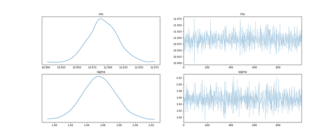
However the slowdown may not be in the model logp being heavy but in it being poorly identified. How do the traces look like after sampling is done?

Nothing alarming to me. No warnings about divergences either.


For comparison here’s a trace plot of the naive model.

I mean pytensor.tensor.vectorize which works just like numpy.

You shouldn’t be compiling a pytensor function yourself, just use pt.as_tensor([-2, -1, 0, 1, 2, 3]) directly instead of that intermediate dummy new_shifts

...
densities = vectorize_graph(density, replace={shift: pt.as_tensor([-2, -1, 0, 1, 2, 3])})
...

You can probably vectorize a bit further along the lines of

densities = log((densities[3:][::-1] - densities[:3]) * [5/9, 3/9, 1/9])

I tried using both pt.vectorize and vectorize_graph. Both versions use

densities = log((densities[3:][::-1] - densities[:3]) * [5/9, 3/9, 1/9])

though I had to do some reshaping for it to work.

The vectorize version (below) required that all inputs are TensorVariable and not TensorSharedVariable. Is there a way to do the switch explicitly? I didn’t find a way how to and did value + pt.shape_padright([-2, -1, 0, 1, 2, 3]) instead. This version was slower than the original one by roughly 10 %.

def _gamma_cdf(mu, sigma, value):
    dist = pm.Gamma.dist(mu=mu, sigma=sigma)
    return exp(pm.logcdf(dist, value))


def _podium_logp(value, mu, sigma):
    cdf = pt.vectorize(_gamma_cdf)
    densities = cdf(mu, sigma, value + pt.shape_padright([-2, -1, 0, 1, 2, 3]))

    densities = (densities[3:][::-1] - densities[:3]) * pt.shape_padright(
        [5 / 9, 3 / 9, 1 / 9]
    )

    return log(sum(densities, 0))

I managed to get the vectorize_graph version working thanks to your advice but it didn’t help either. It was also slower than the original version by 10 % or so.

def _podium_logp(value, mu, sigma):
    dist = pm.Gamma.dist(mu=mu, sigma=sigma)
    shift = pt.scalar("shift")
    density = exp(pm.logcdf(dist, value + shift))

    densities = vectorize_graph(
        density, replace={shift: pt.as_tensor([-2, -1, 0, 1, 2, 3])}
    )
    densities = (densities[3:][::-1] - densities[:3]) * pt.shape_padright(
        [5 / 9, 3 / 9, 1 / 9]
    )

    return log(sum(densities, 0))

Only checking the marginal distributions can mask degeneracy. Check az.plot_energy (the two curves should overlap) for a global summary of the sampling process. Also check az.plot_pair to check pairwise joint distributions (you should ideally have gaussian clouds – look for linear relationships and geometric discontinuities). Also check the number of integration steps that was needed to generate each sample. It’s in idata.sample_stats.tree_depth, no nice plot to make as far as I know – check that it’s not too huge.

If everything really is OK and it’s still slow, try switching the nuts sampler to nutpie, numpyro, or blackjax for free speedups.

Check az.plot_energy

Is a truncated marginal energy distribution a problem? Otherwise looks pretty close to me.
Podium_energy
The truncation is also visible with the naive model so I guess not? The naive model is plenty fast.
Naive_energy

Also check az.plot_pair

Well, it’s not completely white noise but cannot complain.
Podium_pair
I’d say that there’s more correlation with the naive model.

Also check the number of integration steps

The mean is a bit over 2 and the maximum 4

try switching the nuts sampler

I’m already using blackjax. The default sampler was unusable as even a single sample took ~5 minutes

The truncation can be a problem but not necessarily. I see energy plots like often with models I can’t use the default sampler on. Basically the blue curve is the distribution of total Hamiltonian system energy at each sample (kinetic + potential , where kinetic is the momentum sampled from a normal and potential is the logp). Since Kinetic is a normal, the truncation can only result from the logp term. In general these should be transformed to an unconstrained space during sampling so you shouldn’t see this, but it looks like in your case no such transformation occurs. I’m not sure if you’re allowed to manually specify a transformation to a pm.CustomDist, but it might be worth a try if so. Even if you are, I’m not sure what transformation would be appropriate in your case…

Basically when the sampler spends time in those low energy states in the left tail of the distribution it will be doing inefficient exploration.

I have no idea if this is the source of your problem or not, though. All the other diagnostics look fine, so the bottleneck might really be computational. You could try timing the logp and dlogp functions (use model.compile_logp and .compile_dlogp. If dlogp is really the bottleneck you could try a gradient-free sampler like SMC?

You could try timing the logp and dlogp functions (use model.compile_logp and .compile_dlogp.

Yeah it looks like dlogp calls are ~3500 times slower with my custom distribution compared to just using pm.Gamma. logp calls are “only” 60 times slower. Is there a way to check the dlogp graph or manually define the dlogp function? I don’t have high hopes that I could remedy the situation but would be interesting to at least check what the graph looks like. I found pytensor.dprint(pymc.logp()) but couldn’t find and equivalent function for gradients.

Since Kinetic is a normal, the truncation can only result from the logp term. In general these should be transformed to an unconstrained space during sampling

Can there be a transform for the logp in addition to the variable transformations?

The logp functions are saved in the model itself, so you can directly use mod.logp() and mod.dlogp(). But it is more useful to look at the compiled graph, because that’s what you’re actually going to be timing. You can dprint compiled pytensor functions, but PyMC hides them from you a bit like this:

wrapped_f = mod.compile_dlogp()
pytensor.dprint(wrapped_f.f)

As I tried to suggest by the naming, PyMC wraps the underlying pytensor functions it creates with some logic to make passing the outputs of MCMC steps more convenient. For benchmarking/debugging though you need the “raw” function, which is saved in the .f attribute.

One other note about timing, if you are compiling to a non-standard backend (like jax or numba) make sure you time the jitted function. You actually can’t do this with mod.compile_dlogp, you have to use mod.compile_fn:

wrapped_f = mod.compile_fn(mod.dlogp(), mode='JAX')
jax_f = wrapped_f.f.vm.jit_fn

jax_f will be the raw jitted JAX function that you can then use for timings (make sure you run it once before you %timeit to trigger the JIT compilation).

Another useful thing to do is to enable the profiler, you can do this with profile = True in mod.compile_fn(mod.logp(), profile=True), run %timeit, then look at f.profile.summary(). That will show you which operations are consuming the most time.

Variable transformations are only for the logp graph, so I’m not sure what you mean.

For benchmarking/debugging though you need the “raw” function, which is saved in the .f attribute.

Thanks for pointing that out. It didn’t change the outcome however, dlogp calls are still ~3500 times slower with my custom distribution.

One other note about timing, if you are compiling to a non-standard backend (like jax or numba) make sure you time the jitted function.

I tried this but I cannot compile my custom distributions dlogp. I get NotImplementedError: Dispatch not implemented for Scalar Op gammainc_grad_b. Sampling works fine though and I don’t get errors. Does nuts_sampler="blackjax" use something else for calculating the gradients or are there fallbacks in the case of missing implementations?

Another useful thing to do is to enable the profiler, … , then look at f.profile.summary().

Is there a way to get more fine grained info than in the image below? If I understood correctly (by comparing to the appended graph.txt), the profiling currently tells me that almost all of the time is spent calculating the likelihoods and not much else.


graph.txt (8.8 KB)

Variable transformations are only for the logp graph, so I’m not sure what you mean.

Sorry for the confusion, I’m kinda confused myself. I guess what I tried to ask is that I’m using the custom distribution in my likelihood and not in priors and I don’t quite understand what you meant by “manually specify a transformation to a pm.CustomDist”.

I’m using mean-variance parametrization for my underlying gamma distribution and I have defined normal and half-normal priors for mu and sigma, respectively. mu is not constrained and does not get transformed. sigma is transformed to sigma_log__ as it should. Are you talking about some other transformations besides these or am I completely off the tracks? Should there be other transformations in addition to the obvious posterior → log-posterior transformation?