I want to infer the parameter of multivariate Poisson distribution with pymc.
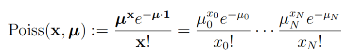
Such multivariate Poisson distribution like this:
An example infer the parameter of multivariate normal distribution like this:
cov_true = np.array([[1., 0.5], [0.5, 2]])
mu_true = np.zeros(2)
data=np.random.multivariate_normal(mu_true, cov_true,100)

textmodel = pm.Model()

with textmodel:
    mu=pm.Normal('mu',shape=(2,))

    vals = pm.MvNormal('vals', mu=mu, cov=cov_true, observed=data)

    idata = pm.sample(1000, random_seed=111)

with textmodel:
    idata.extend(pm.sample(1000, tune=2000, chains=2, random_seed=111))

az.plot_trace(idata)
And I can get the right inference from joint distribution.
But how can I get the same process for multivariate Poisson distribution? Maybe I need such a class name “MvPoisson” like “MvNormal”, but I can’t implement.
I would think you want to simulate data taken from a Poisson that you use for your likelihood function. I tried to modify your code to use the Multivariate Normal Distribution for the priors (I also had it infer the LKJCholeskyCov). I then use an exponential link function for the observed data. It seems to sample OK but plotting the trace returns an error for an infinity value in the standard deviation fit).
rng = np.random.default_rng(1)

num_samples=100
cov_true = np.array([[1., 0.5], [0.5, 2]])
mu_true = [3,3]
mean_samples = np.random.multivariate_normal(mu_true, cov_true,num_samples)
poisson_samples = rng.poisson(np.exp(mean_samples))
textmodel = pm.Model()

with textmodel:

    sd_dist = pm.Exponential.dist(1.0, shape=2)
    chol, corr, stds = pm.LKJCholeskyCov('chol_cov', n=2, eta=2,
    sd_dist=sd_dist, compute_corr=True)

    mu = pm.MvNormal('mu', mu=0, chol=chol)

    counts = pm.Poisson("y", mu=pm.math.exp(mu), observed=poisson_samples)

with textmodel:
    idata = pm.sample(1000, random_seed=111)
# with textmodel:
#     idata.extend(pm.sample(1000, tune=2000, chains=2, random_seed=111))
az.plot_trace(idata)
az.summary(idata)
mean sd hdi_3% hdi_97% mcse_mean mcse_sd ess_bulk ess_tail r_hat
mu[0] 0.450 0.077 0.300 0.591 0.002 0.001 1739.0 1371.0 1.0
mu[1] 1.295 0.053 1.205 1.401 0.001 0.001 1571.0 1480.0 1.0
chol_cov[0] 0.871 0.714 0.125 2.034 0.020 0.015 1590.0 1340.0 1.0
chol_cov[1] 0.244 0.706 -1.190 1.501 0.019 0.018 1485.0 982.0 1.0
chol_cov[2] 1.331 0.770 0.296 2.699 0.023 0.016 1163.0 907.0 1.0
chol_cov_corr[0, 0] 1.000 0.000 1.000 1.000 0.000 0.000 2000.0 2000.0 NaN
chol_cov_corr[0, 1] 0.183 0.401 -0.518 0.895 0.009 0.008 2010.0 1053.0 1.0
chol_cov_corr[1, 0] 0.183 0.401 -0.518 0.895 0.009 0.008 2010.0 1053.0 1.0
chol_cov_corr[1, 1] 1.000 0.000 1.000 1.000 0.000 0.000 1826.0 1606.0 1.0
chol_cov_stds[0] 0.871 0.714 0.125 2.034 0.020 0.015 1590.0 1340.0 1.0
chol_cov_stds[1] 1.502 0.817 0.447 2.886 0.027 0.019 1001.0 1061.0 1.0