Large variance of noise when modeling AR process

I am performing AR(1) process with an intercept using the below equation-
x(t) = a*x(t-1) + c + N(0,s),
where a, c and s are the parameters of the model, and N(0,s) is a normal with s as its variance. I am using ADVI with adam to estimate the parameters, and run the adam till it reaches convergence. I am facing the issue that the variance of Normal distribution is too large even though the prediction of the model is very accurate. Please find the results attached
download (2)

I am using all the points to learn the parameters of the model and then using the posterior distribution of those to perform prediction on the same dataset. Why is the variance large? What can I do to reduce it? Theoretically, it should be small given the predictions of the model are super accurate.

Edit: When I remove the intercept, the accuracy increases but still the variance is very high.
download (3)

Can you try fitting this model with MCMC (NUTS) instead of ADVI and see what kind of result you get? Its pretty common for VI to do a decent job with point estimates but not with posterior uncertainty. Unless your data is prohibitively large, MCMC is generally a better approach for estimating Bayesian models.

I tried running MCMC, it took around 5 hours to run, but the results are almost the same. Below is the model I am running-

with pm.Model(coords=coords, check_bounds=False) as autoregressive_model:

sigma = pm.HalfNormal("sigma", .2)
ar_init_obs = pm.MutableData("ar_init_obs", np.squeeze(u_scale[0:lags,0:features]), dims=("features"))
ar_init = pm.Normal("ar_init", observed=ar_init_obs, dims=("features"))

PAT_true = pm.MutableData("PAT_obs", PAT_obs, dims=("trials"))    

mu2_a = pt.zeros(features)
sd_dist_a = pm.Exponential.dist(1.0, shape=features)
chol2_a, corr_a, stds_a = pm.LKJCholeskyCov('chol_cov_ar', n=features, eta=2,
sd_dist=sd_dist_a, compute_corr=True)
A_ar = pm.MvNormal('A_ar', mu=mu2_a, chol=chol2_a, shape=(features))

sigmas_Q_ar = pm.HalfNormal('sigmas_Q_ar', sigma=1, shape= (features))
Q_ar = pt.diag(sigmas_Q_ar) 
intercept = pm.Normal("intercept", mu=0, sigma=1, dims=("features"))
def ar_step(x, A, Q, intercept):
    mu = A*x 
    #mu = pm.math.dot(A,x) + intercept
    next_x = mu + pm.MvNormal.dist(mu=0, tau=Q)
    return next_x, collect_default_updates(inputs = [x, A, Q, intercept], outputs = [next_x])

ar_innov, ar_innov_updates = pytensor.scan(
    fn=ar_step,
    outputs_info=[ar_init],
    non_sequences=[A_ar, Q_ar,  intercept],
    n_steps=trials-lags,
    strict=True,
)

ar_innov_obs = pm.MutableData("ar_innov_obs", u_scale[lags:,0:features], dims=("steps","features"))
ar_innov = autoregressive_model.register_rv(ar_innov, name="ar_innov", observed=ar_innov_obs, dims=("steps","features"))

ar = pm.Deterministic("ar", pt.concatenate([ar_init.reshape((1,features)), ar_innov], axis=0))
ar_obs = pm.Deterministic("ar_obs", pt.concatenate([ar_init_obs.reshape((1,features)), ar_innov_obs], axis=0))

There are in total 8 features and the graph which I displayed is for one of the features. Is there any issue with the above modeling process?

Below is the distribution of sigmas
sigmas

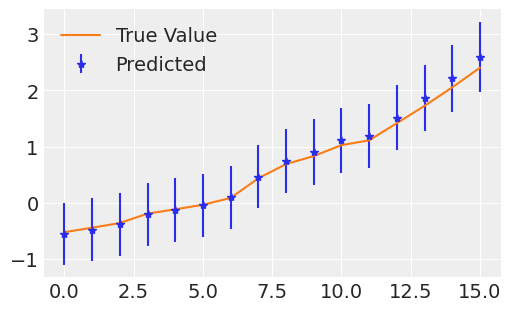
Below is the prediction for feature 0
down1

Why do you say this? You are using a long-tailed distribution for the standard deviation of size of the AR coefficients (Exponential), while also trying to estimate a dense correlation matrix between them. There’s a lot of prior uncertainty in your model that’s going to linger unless you have mountains of data to provide the model. I’d do some parameter recovery exercises using data generated from the priors to study how much data your model needs to achieve a desired level of accuracy.

As for modeling speed, I recommend always using a JAX sampler with scan-based models. I see enormous speedup when I do this. Also since Q is diagonal, you can just make your noise term pm.Normal.dist(mu=0, tau=sigmas_Q_ar). This will avoid expensive matrix inversion operations at every step of your scan.

Also, since (I think?) your model is just an AR(1), you know that the space of stationary parameters is just the interval (-1, 1). I’d try pumping your estimated parameters though a deterministic function, like pt.tanh, to force them to stay on that stationary interval. That should also speed up sampling, because it will rule out exploding trajectories (especially if “steps” is large). If your AR order is greater than 1, it’s harder, and I would be using strongly regularized priors.

Finally, have you looked at the built-in pm.AR distribution? Since you don’t have an MA component, there’s no need to do this state-space setup.