Linear regression with Generalized extreme value distribution

[alok]

Hi,
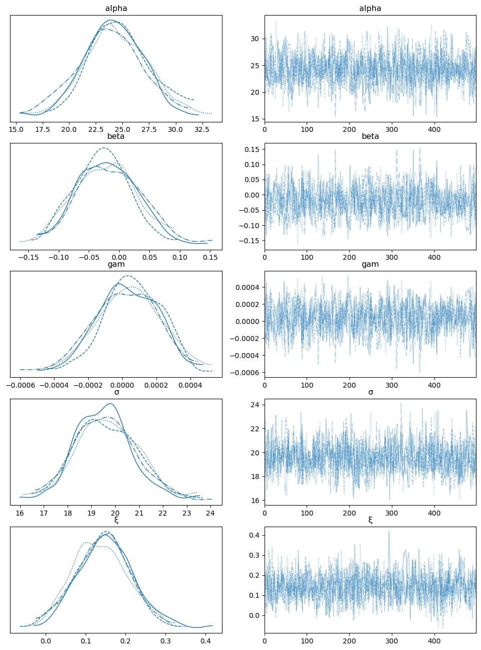
I am quite new to Bayesian Liner regression. I want to perform linear regression using Generalized extreme value (GEV) distribution. My code is working well while trying to estimate the three parameters of GEV. However, I am getting wrong values when I am assuming the location parameter (mu) as a function of time to account for nonstationary. The rhat statistics is larger than 1.01 for all the parametrs and I am getting a single value.
Below is my code:

X = np.linspace(1, 276, 276)
X = X.astype(int)
df1 = pd.read_csv('Datapy.csv')
[Datapy.csv|attachment](upload://ladV0IWHHMafHpK7VjaaOU6CzRh.csv) (2.1 KB)


###################################
with pm.Model() as model:
    # Priors
    alpha =pm.Normal('alpha', 0, 100)
    alpha = alpha.astype(int)
    beta = pm.Normal('beta', 0, 100)
    beta = beta.astype(int)
    gam = pm.Normal('gam', mu=0.0, sigma=100.0)
    gam = gam.astype(int)
    
  
    σ = pm.HalfNormal("σ", sigma=21)
    ξ = pm.Normal("ξ", mu=0.0, sigma=0.35)
    # Expected value of outcome
    μ = alpha + beta*X +gam*X^2
   
    # Estimation
    gev = pmx.GenExtreme("gev", mu=μ, sigma=σ, xi=ξ, observed=df.r)
#####################################################################    
    
idata = pm.sample_prior_predictive(samples=1000, model=model)
az.plot_ppc(idata, group="prior", figsize=(12, 6))
ax = plt.gca()
az.plot_posterior(
    idata, group="prior", var_names=["alpha", "beta","gam","σ", "ξ"], hdi_prob="hide", point_estimate=None
);

######################################################
with model:
    trace = pm.sample(
        500,
        cores=4,
        chains=4,
        tune=2000,
        initvals={'alpha':0.92, 'beta': -2.5, "gam": 0.9, "σ": 1.0, "ξ": -0.1},
        target_accept=4,
    )

I have uploaded the data if you want to try. Any help would be greatly appreciated.

Thanks,
Alok

[ccaprani]

Can you just check a couple of things?

I think the exponent here should be **, otherwise you’ll get a bitwise operation.

μ = alpha + beta*X +gam*X^2

ξ = pm.Normal("ξ", mu=0.0, sigma=0.35)

This is a wide prior for ξ and could be giving trouble - trying reducing it to maybe sigma=0.1 and if that runs, bring it back up gradually then to a suitable prior.

[alok]

Hi,
Thank you so much for your reply. I tried both the suggestions you pointed out. I also tried ξ and gam with sigma = 0.01. However, there is no change in the results.

Please let me know if I should try something else!

Thanks

[ccaprani]

Hmmm…it’s a really interesting use-case, and so I would like to figure this out. I can’t access your data (can you make available?), but perhaps a useful test is to see if your generative model can generate data similar in form: that is - what do your prior predictive checks look like?

[alok]

Datapy.csv (2.1 KB)

Hi,
I have uploaded the dataset. Please let me know if you still have problem accessing the data.

Thanks,
Alok

[ccaprani]

Got it - give me a couple of days!

[ccaprani]

Ok, well I’m a sucker for a problem, so here goes.

X = np.linspace(1, 276, 276)
X = X.astype(int)
df = pd.read_csv('Datapy.csv')

with pm.Model() as model:
    # Priors
    alpha =pm.Normal('alpha', 20, 5)
    #alpha = alpha.astype(int)
    beta = pm.Normal('beta', 0, 1)
    #beta = beta.astype(int)
    gam = pm.Normal('gam', mu=0.0, sigma=0.1)
    #gam = gam.astype(int)
    
    σ = pm.HalfNormal("σ", sigma=10)
    ξ = pm.Normal("ξ", mu=0.0, sigma=0.1)
    # Expected value of outcome
    #μ = pm.Normal("μ", mu=20, sigma=5)
    μ = alpha + beta*X + gam*X**2
   
    # Estimation
    gev = pmx.GenExtreme("gev", mu=μ, sigma=σ, xi=ξ, observed=df.r)

idata = pm.sample_prior_predictive(samples=1000, model=model)
az.plot_ppc(idata, group="prior", figsize=(8, 3))
ax = plt.gca()
ax = plt.gca()
ax.set_xlim([-50, 200])
ax.set_ylim([0, 0.04]);

az.plot_posterior(idata, group="prior", var_names=["alpha","beta","gam","σ","ξ"], hdi_prob="hide", point_estimate=None, figsize=(8, 3));

with model:
    trace = pm.sample(
        500,
        cores=4,
        chains=4,
        tune=2000,
        initvals={'alpha':22, 'beta': -0.01, "gam": 0.0, "σ": 15.0, "ξ": 0.2},
        #initvals={'alpha':0.92, 'beta': -2.5, "gam": 0.9, "μ": 50, "σ": 3.0, "ξ": -0.1},
        target_accept=0.9,
    )
idata.extend(trace)

az.plot_trace(idata, var_names=["alpha", "beta", "gam", "σ", "ξ"], figsize=(12, 16));

The main thing was to choose more reasonable priors. Building up from a single GEV distribution fit showed that the X wasn’t so influential: beta is small and gam is close to zero. Also, the target value should be < 1.0 and it’s good to let the sampler select its own starting point, at least initially.

Compare the prior predictive check for the case for no linear dependence with the one for the quadratic dependence with these much tigher priors. It gives a good idea how important priors are here.

No linear dependence (7 secs)
Samples great.

Linear dependence (8 secs)
Needs a sensible prior for alpha and beta.

Quadratic dependence (37 secs)
Samples badly - can be lots of divergences, even with tight priors for gam, reasonable initvals and a higher target_accept.

With integers
Turning even just alpha to an astype(int) causes the sampling to go nuts (haha!) - it takes about 450 seconds then and looks just awful. DO you really need these parameters to be ints?

[alok]

Thank you so much @ccaprani . I guess “astype(int)” was creating the problem. I have one last question. How did you know that beta and gam should have tighter priors or How do you approach to this type of problem when you have no information about prior?

Do you check the prior predictive or Do you try to fix one coefficient first? It is difficult to start when you have a single value for each parameter.

Thanks,
Alok

[ccaprani]

You’re welcome @alok !

Anytime there is a complex problem like this, just try and break it down to its simplest case and then gradually rebuild towards the intended model. For this one, I commented out the linear regression bit and did a straight GEV fit first. Even that had trouble and so I adjusted the priors to get in the right zone (see PPC plot). Then add back in the linear dependence (beta, since alpha is just mu, i.e. the offset). Here, I started with beta priors being very tight, so similar to the ordinary GEV fit, then widen until PPC plot looks ‘reasonable’ (compare my two with your one which covered a very wide domain). Same with gam.

I’m still in awe of the people doing much more complex models though. Really not sure how they manage! I guess practice & experience helps them. Plus a good principled Bayesian workflow!

[alok]

Thanks for the help!