Lognormal constraint poor convergence

Hi, there have been a few questions about the LogNormal already, but I feel nothing as straightforward as this:

import pytensor.tensor as pt
import pymc as pm

s, loc, scale = 0.94, -32, 152   # from a scipy fit

with pm.Model() as model:
    # q = pm.Uniform("ais", lower=loc, upper=1000)  # this converges fine
    q = pm.Uniform("ais", lower=loc-10, upper=1000) # this doesn't !
    q = pt.clip(q, loc+1e-9, 1e9)
    log_lik = lambda x: pm.logp(pm.Lognormal.dist(mu=np.log(scale), sigma=s), x-loc)
    pm.Potential("constraint", log_lik(q))
    trace = pm.sample()

As long as I stay strictly in the definition domain of the lognormal, this converges fine, otherwise, it does not (the example above has about 120 divergences on four chains). In my real model, the q parameter is the result of a more complex calculation and cannot be chosen as it pleases the sampler. I’d just like to assign the probability of going there something small, close to zero when less than the threshold, and lognormal otherwise. I tried to transform q in various ways besides clip, to no avail. Any idea how to achieve this?

PS: the result looks OK, but the convergences are not a good sign nonetheless

import arviz as az
from scipy.stats import lognorm
axes = az.plot_trace(trace)
x = np.linspace(*axes[0, 0].get_xlim(), 100)
dist = lognorm(s, loc=loc, scale=scale)
y = dist.pdf(x)
axes[0, 0].plot(x, y, "r")

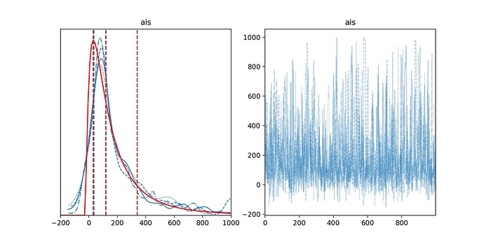
I think the difference between the two cases, is the clip introduces a discontinuity / flat region in the gradient but does not avoid the sampler for seeing it, whereas your original uniform completely avoids the impossible region.

I guess so. While replying you, I found a reasonable workaround. I don’t really need to have that particular log-norm. I only wanted to target a given set of quantiles [0.17, 0.5 , 0.83] with associated values [ 30., 120., 340.]. The above-mentioned distribution is the one that best fits these quantiles but it don’t mind if there were a low-probability, thin tail further down the negative values. So in the end I used ifelse to join a Normal distribution for values below the median, to avoid the sharp low bound of the log-normal:

from pytensor.ifelse import ifelse

with pm.Model() as model:
    q = pm.Uniform("ais", lower=-200, upper=1000)
    pm.Potential("constraint", ifelse(
        pt.le(q, observed_values[1]),
        pm.logp(pm.Normal.dist(observed_values[1], observed_values[1]-observed_values[0]), q),
        pm.logp(pm.Lognormal.dist(mu=np.log(scale), sigma=s), q-loc),
       ))
    trace = pm.sample()

And below is the result. In red the original fitted log-normal, and dashed red the target quantiles vs blue dashed line the posterior quantiles. It’s satisfying enough to me (I guess I can also join further left and tune the tail to my taste).

Thanks for the stimulus.

You could directly use a pm.Mixture here instead of the potential?

Could I ? I guess I could define the mixture, but how to define the likelihood then? I wouldn’t even know how to use a simple LogNormal directly without a Potential. If you have a suggestion that’d be most welcome.

Looking at the code you’ve posted more carefully, I honestly don’t understand what’s going on, so I retract my suggestion. I wrote out some code for a CustomDist for loc-scale parameterization of a LogNormal in the first model, but now I see you’re not actually providing data there and the parameters are fixed. It’s fundamentally not a generative model, so I guess you’re locked into using Potential.

Same goes for the second model. The data are being used as parameters of the normal – why?

Thanks for the discussion @jessegrabowski . The short answer is that I am not trying to estimate the parameters of the log-normal distribution, and the ais Uniform prior is a placeholder for a more complex model.
I have a larger model that simulates sea level rise based on historical datasets, for which the Bayesian likelihood definition is straightforward (my model is the smooth trend, what is the chance of measuring an observation given “noise” occuring in nature, and measurement errors). Now for the projections into the future, I also want to include other constraints that come from independent estimate with physically-based models. They are not direct observations. And these estimates tend to produce a log-normal looking distribution for the Antarctic Ice Sheet (low- but non-zero probability of a high contribution to sea-level from Antarctica), which I sum-up with a known log-normal distribution. I’m not sure what is the best way of integrating that knowledge in the model. If I had only one number (the ais term in the simple model above), I’d use it as a prior distribution. However, the Antarctic contribution comes from an equation involving a few other parameters and exogenous variables (surface air temperature timeseries). So using Potentials is the best (and only) way I found so far. Please let me know if you have a better suggestion.

EDIT: the example above shows that if I have no other information (a uniform prior, no other constraints), then the posterior converges toward the specified log-normal. Now presumably it will also compose nicely along with additional constraints.

I’d have to know how all the pieces fit together to make forecasts. As an example which might be way off base, say I had time series data x_t which is determined by some exogenous process z_t, plus a local-linear trend:

\begin{align} x_t &= \beta z_t + \eta_t \\ \eta_t &= \eta_{t-1} + \alpha_{t-1} \\ \alpha_t &= \alpha_{t-1} + \zeta_t \end{align}

Where \eta_t is the (conditional) level of the series x_t, and \alpha_t is the “velocity” of change of the level. It’s a smooth trend because there’s no error term on \eta_t, only on \alpha_t. You could then define y_t = x_t + \xi_t as a measurement error process.

Anyway, If I was going to forecast this I couldn’t, because to know x_{t+h} I need to know z_{t+h}. If that first line of the equation wasn’t there, I could just iterate on random draws from \zeta_t \sim \text{Whatever} and forecast as far forward as I like.

If I had a secondary model for z_t, though, I could just directly fuse the two models together to make forecasts. The setup would be:

  1. Have the above model of x_t | z_t
  2. Estimate using data x_t, z_t, obtain posterior samples idata_1
  3. Have some model of z_t.
  4. Write a 2nd pymc model which replaces z_t with data generated by my model from step (3), and recycles the posterior parameters obtained in step (2).
  5. Use pm.sample_posterior_predictive to combine the two models and obtain forecasts

So maybe this is a bit rambling, but the point was that because I started from the model that connected x_t and z_t , I could do the forecasts in a generative fashion. I guess in your case, x_t is sea level and z_t is antarctic ice-sheet. It doesn’t seem like you have z_t in your initial model. Nothing stops you from doing exactly what I’ve laid out here though without that modification – just estimate the time series x_t without z_t, then introduce z_t afterwards. That should be fine (as long as the posteriors you obtain on the x_t model are conditionally independent of z_t), as long as you can write down the relationship between x_t and z_t.

Hi @jessegrabowski , thanks for the detailed answer. At first glance it seems a little far fetched indeed, because the situation I am facing already occurs without all that complexity.
Here is the simplest version of a full model for which I already encounter the problem I mentioned earlier:

T = ...  # temperature time-series starting in 1900, with 0 around 2000s, and heading to around 2 in 2100
with Model() as model:
  q = HalfCauchy("q", .15)  # rather large (ignorant) prior
  a = Normal("a", 0, .5)  # rather large (ignorant) prior
  c = Normal("rate_1993_2018", 0.25, .06)  # prior for 1993 to 2018 linear trend in mm / yr
  rate = q*T^2 + a*T + c  # a quadratic model on the rate of sea level
  slr = pt.cumsum(rate)
  pm.Normal("slr_1900_to_1990", slr[90] - slr[0], .3, observed=.4)  # obs constraint on cumulative SLR in mm
  pm.Potential("slr_2005_2100", pm.logp(...., slr[200] - slr[105]))  # the log-normal potential discussed previously
  pm.sample()

Now this model is still a small part of the full model, which include other contributions to sea level and also includes local observations (tide gauges, satellite, GPS…), spatial patterns, spatially-correlated ocean variability and other effects. But this does not really matter here. The point is, how to include the log-normal knowledge in the model, when I cannot use that directly as prior? Well, in this case I could resolve this analytically by integrating over konwn T, using slr_2005_2100 as a true log-normal prior, and making q a deterministic parameter that depends on slr_2005_2100, a and c. That way I could get rid of the potential. That should be equivalent as far as I understand it…though I’m a bit wary of doing that kind of analytical inversion. And it won’t be possible if I update my quadratic model to something else. Anyway, I feel we are talking about two different situations.

In the example above, I just use a Normal distribution as constraint and that is fine. Now another way of seeing the question is, what happens when my measurement process is more complex, skewed to one side. I think here it would look like a log-normal distribution mirrored between model and obs. I guess I am just having trouble to find the analytical parameters to the log-normal distribution that match the reflected log-normal, i.e. moving from pm.Lognormal.dist(mu=np.log(scale), sigma=s), q-loc) to pm.Lognormal('obs', ..., q, ..., observed=...)

I guess I’m still struggling with why, for example, rate is transformed into just a single point. Shouldn’t the rate be inferred conditional on the observed sea level in every year? Calling S_t the sea level, I would expect you model something like S_t = e^{r_t}u_t, with u_t \sim \text{LogNormal}(0, \sigma_u) so that \ln S_t = r_t + \varepsilon_t is normally distributed. Then you just proceed with a normal PyMC model, plugging in the sea levels as observed, and modeling r_t = c + qT_t^2 + aT_t .

The point of my big post above was to try to elicit these functional relationships, because I think it will get you to a better model in the end. I agree you could make everything into a potential, but it’s not at all clear to me how it all hangs together (though I admit I’m being somewhat nosy and you might be perfectly happy with you model, in which case I’ll drop it)

Yes, sea level should be conditional on observed sea level every year, but as it stands, it only takes a few metrics, such as over SLR during the 20th century, then present-day rate, and indeed some projections to 2100. The reason is to avoid having to deal with complex auto-correlation for now. I was quite happy with the model until recently but I am currently not because of the divergences and shows some variation from one chain to another in the tails (this can be reduced with target-accept, but still). I’m happy to find a formulation without Potential, and am trying to follow your logic, but I’m also struggling to come the other way. Here what you are saying is that I should use a different model :slight_smile: ?! What if my quadratic formulation had some physical basic, and I simply wanted to have my parameters distributed in such a way that my outcome is log-normal ? I mean, it’s not like the quadratic relationship between SLR and temperature is established (it’s not and indeed can be changed), but I’d think an exponential of a quadratic would be further remote from reality and it would be hard to find a physical justification for such a form.

Don’t these lines imply that you’re modeling the log of sea level as quadratic?

  rate = q*T^2 + a*T + c  # a quadratic model on the rate of sea level
  slr = pt.cumsum(rate)

Otherwise I would expect slr = (1 + rate).cumprod()

Not really, no. Cumsum is a cumulative sum of yearly increment. The rate is in mm/yr, and I am modelling this rate as a quadratic function of temperature. The cumulative sea level rise over many years (in mm, say) is the time-integral of the rate, or cumulate sum. In equations, that means rate = d(slr)/dt and slr = \int_0^t rate(t, T(t)) dt. If the temperature were a linear function of time, the cumulative sea level would become a cubic function of time. Sorry if I take for granted things I have always considered under the same light.

EDIT: I see you are probably an economist and used to relative rates of growth (which accumulate as a product over time). Whereas in climatology when we say sea level rise, or rate of sea level rise, we always talk about arithmetic series.