Lognormal distribution for donations

[danielbarco]

Dear pymc experts,

I am trying to compare two sets of donation data that were generated in a A/B test. The values are donation income (revenue).

data = [120.0, 500.0, 0.01, 40.0, 1000.0, 150.0, 1500.0, 13.0, 200.0, 3000.0, 200.0, 45.0, 221.0, 20.0, 100.0, 60.0, 400.0, 20.0, 250.0, 60.0, 100.0, 60.0, 30.0, 120.0, 40.0, 60.0, 100.0, 1500.0, 450.0, 1.0, 250.0, 200.0, 100.0, 100.0, 300.0, 120.0, 45.0, 120.0, 200.0, 150.0, 120.0, 50.0, 201.0, 50.0, 200.0, 200.0, 50.0, 200.0, 1.1, 80.0, 1400.0, 20.0, 50.0, 250.0, 60.0, 60.0, 60.0, 150.0, 20.0, 100.0, 120.0, 20.0, 550.0, 45.0, 250.0, 250.0, 15.0, 60.0, 300.0, 20.0, 30.0, 400.0, 200.0, 60.0, 400.0, 500.0, 30.0, 50.0, 250.0, 50.0, 5.0, 1.0, 1.0, 50.0, 50.0, 100.0, 120.0, 60.0, 5.0, 5.0, 30.0, 30.0, 60.0, 15.0, 50.0, 100.0, 200.0, 100.0, 100.0, 50.0, 100.0, 50.0, 50.0, 550.0, 75.0, 100.0, 250.0, 20.0, 1000.0]
idx = [0, 1, 0, 0, 1, 1, 1, 1, 0, 1, 1, 0, 0, 1, 1, 1, 0, 0, 0, 1, 1, 0, 1, 1, 1, 0, 0, 0, 1, 0, 1, 1, 1, 0, 1, 1, 0, 0, 0, 0, 1, 0, 1, 1, 0, 1, 0, 0, 0, 1, 0, 1, 0, 1, 0, 0, 0, 1, 0, 0, 0, 0, 1, 0, 1, 1, 1, 1, 0, 0, 0, 0, 0, 0, 1, 1, 1, 0, 0, 1, 0, 0, 1, 1, 0, 1, 0, 1, 0, 0, 0, 1, 1, 0, 0, 1, 1, 1, 0, 1, 0, 1, 0, 1, 0, 1, 0, 1, 0]

I have tried to model the data using a lognormal distribution, which ran without divergences.

with pm.Model() as model:   
   
   µ_log = pm.Normal('µ_log', mu = 0, sigma =  2, shape = groups)    
       
   sigma = pm.HalfNormal('sigma', sigma = 4, shape = groups)

   y_hat = pm.Lognormal('y_hat', mu = µ_log[idx], sd = sigma[idx], observed = data)
   
   µ = pm.Deterministic('µ', np.exp(µ_log))

   mode_log = pm.Deterministic('mode_log', µ_log - sigma ** 2)
   mode = pm.Deterministic('mode', np.exp(mode_log))
   median = pm.Deterministic('median', np.exp(µ_log))
   
   diff_of_modes = pm.Deterministic('diff of modes', mode[1] - mode[0])
   diff_of_median = pm.Deterministic('diff of median', median[1] - median[0])
   
   trace = pm.sample(10000, tune = 10000)
   ppc = pm.sample_posterior_predictive(trace, samples = 20000, model = model, var_names=['µ','µ_log', 'y_hat', 'mode'])
   pm.traceplot(trace)

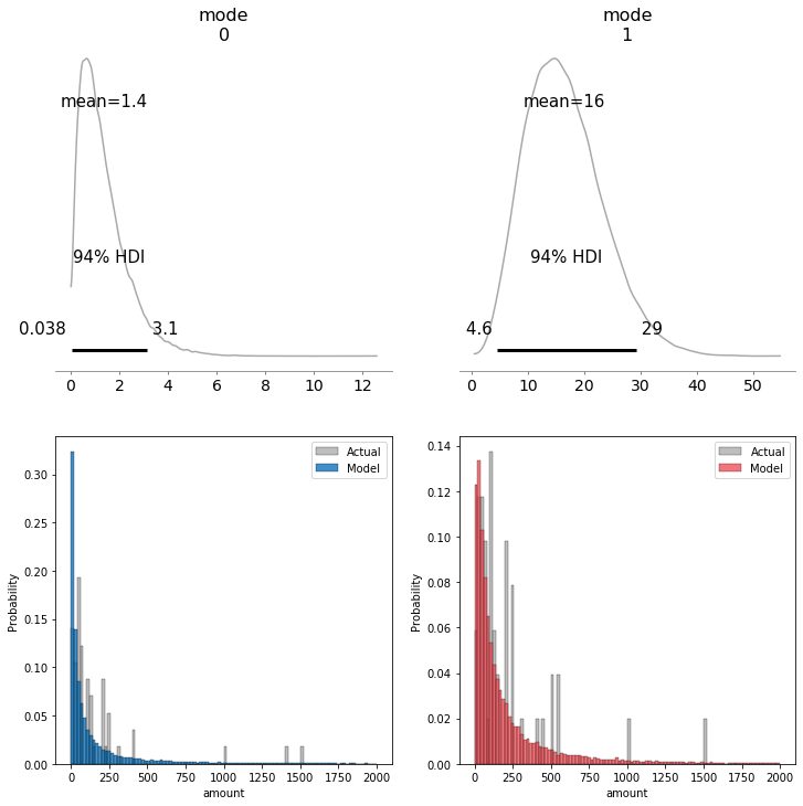
However I noticed, that the estimated mode does not seem to reflect the data very well. I would have expect the most likely values for the mode to be 50 or 100, however the modes are well below that.

Do you have any suggestions on how I could improve this model? Can you spot any errors in my code or thought process?

[ricardoV94]

Are you sure about the mode formula? The posterior plots of the exponentiated mu look very different

[chef1075]

Is there a reason you’re passing in the raw data? Have you thought about standardizing the data ( data ~ Norm(0, 1) ) so the sampler has an easier time?

I’m not sure that will help you with your question about the mode, but it make make specifying the parameters easier.

[danielbarco]

Thank you for your response. I took this formula from Wikipedia to calculate the mode like this:

mode_log = pm.Deterministic('mode_log', µ_log - sigma ** 2)
mode = pm.Deterministic('mode', np.exp(mode_log))

Do you have any suggestions of what might be wrong?

[ricardoV94]

Just checked your plots above, maybe the mode is not so unusual. The lognormal is very skweked. The plot on Wikepedia illustrates this very well.

[danielbarco]

Thank you @ricardoV94. It is exactly this plot which made me question the model. I am struggling to understand how the modeled modes are not around 50/100, the most frequent donated values. Here I have plotted values below 500.

As far as I understand the mode should reflect the most frequent/ probable value. This does not seem to be the case (50 is not within the HDI of mode0 or mode1). This is what is confusing me. Would you choose the lognormal distribution for this data or is there a better fit?

[KyleJCaron]

One thing I’m noticing in your posterior predictive samples of y_hat is that there are some really extreme values, despite the max of your dataset not being much greater than $2000

You could try is to have more informative priors - one thing I’ve done in the past is use an informative/narrow TruncatedNormal distribution around sigma, and use prior predictive sampling to see what the possibilities are. If you restrict sigma to a more narrow range and limit the frequency of those extreme values in the prior predictive samples you could end up with better inference.

Definitely recommend sampling fake data from a log normal distribution and seeing if it’s possible for it to look representative of your dataset.

In terms of distribution choice, I’ll leave that up to the experts, hopefully someone with a better background can chime in with a good recommendation

[danielbarco]

Thank you @KyleJCaron. I have looked more closely at my distribution in log space and realised, that a log student t distribution seems to be much more representative (looking at the distribution in log scale).

For now I have come up with the following, where the difference in distribution can only be shown with a 80% HDI:

with pm.Model() as log_studt:   
    
    µ_log = pm.Normal('µ_log', mu = 5, sigma =  1, shape = groups)    
        
    sigma = pm.HalfNormal('sigma', sigma = 0.5, shape = groups)
    
    nu = pm.HalfNormal('nu', sigma = 3, shape = groups)

    y_hat = pm.StudentT('y_hat', mu=µ_log[idx], sigma=sigma[idx], nu=nu[idx], observed = np.log(data))
    
    diff_of_µs = pm.Deterministic('diff µs', np.exp(µ_log[1]) - np.exp(µ_log[0]))

    trace = pm.sample(10000, tune = 10000)
    ppc = pm.sample_posterior_predictive(trace, samples = 20000, model = log_studt, var_names=['µ_log', 'y_hat', 'diff µs'])
    pm.traceplot(trace)

These results seem possible:

If you spot any errors/ elements with room for improvement please do let me know. Thank you all for your help.

[KyleJCaron]

@danielbarco

If you spot any errors/ elements with room for improvement please do let me know. Thank you all for your help.

Oh nice, your values for sigma look much better! Good idea to choose a studentT and ignore some of those extreme values. I think my one concern is that you’re limiting yourself to the 80% HDI, which tells me you might be seeing problems in the posterior predictive from that student T, but my guess is that your parameter inference might be close to reality. So I’d guees parameter inference might be good enough (you could sample fake data and fit on it to confirm), but if you were to do bayesian decision analysis on your posterior predictive you might want to do some more simulation work to validate things play out smoothly.

I mentioned before I don’t have a great background to be recommending different distributions, but I did some research this past weekend since I had a similar problem and you could also try the following solutions (in case you run into some problems in the future)

• You could try using the Inverse Scale Chi-Sq / Normal Conjugate distribution to model the log scale parameters of your data, and then use those params to calculate whatever you need. This would give you a nice speed up as well (see section 3.3 of Bayesian Data Analysis 3). This solution also allows you to set strongly informative priors on sigma
• You could try a gamma-gamma distribution (see Bruce Hardie’s paper on it). This would also be useful if you have multiple donations per user (but I’d guess that might not be so common). I’d guess there’s also something there with using a regular gamma distribution to model donation amounts but I’m not too familiar