I have a dataset that follows a hurdle lognormal distribution, so I am trying to use pm.HurdleLogNormal as my likelihood function. My initial model is quite simple (I’ve removed any regression coefficients): I have only parameters for psi, mu, and sigma. Model sampling seems to run just fine, and my resulting parameter posteriors seem reasonable; if I sample from the posteriors myself, the resulting data looks roughly how I would expect it to. But when I run sample_posterior_predictive and then plot_ppc, the tails of the posterior predictives are way too long with respect to my observed data. Is there something I am missing with respect to modeling the lognormal distribution?
Model code:
with pm.Model() as hurdlelognormal_model:

    psi = pm.Beta("psi", alpha=3.25, beta=3.25)
    mu = pm.Normal("mu", mu=3.5, sigma=0.5)
    sigma = pm.HalfNormal("sigma", sigma=0.5)

    obs_ = pm.HurdleLogNormal(
        "obs_",
        psi=psi,
        mu=mu,
        sigma=sigma,
        observed=obs,
    )
In order to check if the lognormal distribution is an adequate choice, I filtered my dataset to just the non-zero records, took the log, then created a model using a normal likelihood. Running that simple model results in the following PPC plot, which seems to produce a much better representation of my data! If this works, shouldn’t the lognormal likelihood with the untransformed dataset work? I would just continue building the model with this normal likelihood, but there is no “Hurdle Normal” distribution available.
If y is a vector of strictly positive values, then fitting y ~ lognormal(mu, sigma) will give you the same posterior for mu, sigma as fitting log(y) ~ normal(mu, sigma), assuming you use the same priors. To see that, fit just the normal and lognormal models with the zeros removed.
The lognormal model with zeros removed won’t give you the same posterior predictive inferences as the hurdle model. For example, the hurdle model lets you return zero values. You can’t really plot a density for a mixed discrete/continous model like a hurdle model because there’s non-zero probability mass assigned to a point. You can plot something like a histogram, but it’s misleading given the concentration at zero and the bin width of histograms. Or you can just take the zeros out of the first plot to see if it has the same shape as the second plot.
Thanks for the response. This all makes sense to me, and the parameters do match as expected between those 2 models (y ~ lognormal(mu, sigma) and log(y) ~ normal(mu, sigma). What I am stuck on, though, is why the posterior predictive for the hurdle model (the 2nd and 3rd screenshots I have shared) are far too positive in comparison to the observed data when the posterior predictive for the normal model is reasonable.
A follow up question is, for the normal model, what would I need to add to the model in order to capture the irregularity in the observed data? In other words, the observed data (black) has peaks and valleys above and below the normal distribution, but the posterior predictives (blue) hardly vary from the normal distribution.
Aren’t you seeing an artifact of plot_ppc? perhaps some kernel density estimation that fails with all the zeros in your posterior predictive?
You can try to exclude the zeros of the posterior predictive (not the fit) and call plot_ppc again. You may also need to exclude the zeros of idata.observed_data after fit if there’s a similar thing going on with the observed data.
Ah I see what his point was, but I don’t think it’s an issue with the plot_ppc plot. Some plots of just one prediction shows the same concern, that the posterior predictive has far too long of a tail. The maximum in the observed data in this case was ~17,500.
exp is just a harsh mistress. The distribution produced by your normal model has a right tail out to about 15, and exp(15) = 3e6, which is the scale that you saw in your lognormal PPC. Looking at the box-and-whisker plot, the max value is about 1.4e5, and ln(1.4e5) = 12. So the scales are the same.
I have also been shocked by outputs like this when using lognormal likelihoods. You have to be more judicious about what you plot, or switch to something less explosive.
I see your point. But if the data follows a lognormal distribution, shouldn’t lognormal be the best choice for the likelihood? Perhaps a “Hurdle Normal” with transformed data would be a better choice, but I don’t see that as a distribution option.
Or am I just not capturing the data generating process well enough (ie if the parameter posteriors were tighter, these crazy outliers wouldnt appear)?
Well my point is that both models are the same, so I don’t know what you mean by “best choice”. Just that you judge the log-scaled data to be more aesthetically pleasing. You could address this by not plotting the long tails.
To the second question though, I would focus on running prior predictive simulations. I suspect if you run your current model, you will not be happy with the results. This is a signal that your priors are too flat.
Is there something I am missing with respect to modeling the lognormal distribution?
…
Or am I just not capturing the data generating process well enough (ie if the parameter posteriors were tighter, these crazy outliers wouldnt appear)?
One thing that is helpful to remember is that the mu you plug into the LogNormal is on the log scale, not the natural scale that your data is in. The other weird bit is that the mean of the LogNormal depends on both mu and sigma. The formula for the expected value of the LogNormal is:
exp(\mu + \frac{\sigma^2}{2})
So the mean of the resulting distribution is always higher than what you specify with the prior on mu, even accounting for the exponentiation. It’s very unintuitive to set priors on this guy. In your case, a prior centered around 3.5 on mu means that the LogNormal prior must be north of 33. I suppose that could be reasonable but given your surprise, lowering that might be helpful.
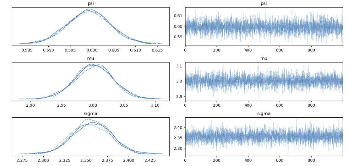
Thanks for the input, all! Everything in the past comments makes sense, but there is still a sticking point for me. The posteriors for the parameters mu and sigma consistently come back centered around ~3 and ~2.3. Clearly these parameters lead to a long tail–longer than that of the observed data. I consider these to be “wrong” because they generate posterior predictives that are skewed far too positively; this is untenable because predictions down the line will lead to ludicrous values. I understand the nature of the lognormal distribution can lead to longer tails, but lognormal seems to be a good choice for my observed data (based on log(observed) looking very close to normal on a histogram). So my questions regarding this and related to the last few comments are
Everyone mentioned changing the priors, but how much could different priors really help at this point? I’ve used various data samples, up to 300,000 records, and the posteriors are more or less unchanged.
If I assume my priors are “good enough” (maybe this is a crap assumption based on an answer to 1….), what would your next steps be to improve this model?
I find it easier to think two ways about lognormal priors. First, with right-skew as in lognormal, means will be higher than medians. The lognormal median is \exp(\mu), so if you’re thinking probabilistically, half the values are below \exp(\mu) and half above and they fall symmetrically around \mu on the log scale. The other way to think about them is that the error are symmetric around 0 on the log scale. That makes odds of 2:1 (2) and odds of 1:2 (0.5) symmetric—they’re 1 and -1 on the log2 scale.
Bayes has the really nice property that if the data really follows the target distribution, then inference will be calibrated. That’s why @ricardoV94 was suggesting the problem is in the model. I wrote a blog post about the calibration issue before Gelman turned off MathJax, but hopefully it’ll still be somewhat readable (otherwise read the simulation-based calibration checking papers, which are based on these properties):
If you have 300K data points and aren’t seeing examples in the tail, that’s even more evidence that the lognormal model is wrong. You could take the log of your data and do a test for normality (or just apply the cdf and plot a histogram, which should look uniform).
The same way that the normal is useful when an effect is the sum of a bunch of independent effect (errors are additive and independent of the value), the lognormal is useful when the effect is the product of independent effects and error is multiplicative (i.e., proportional to value).