Making a query for a simple BN made in PYMC3

rghelichi · February 5, 2019, 2:16pm

I successfully made the student BN example with PYMC3. It seems it gives the general answer correctly.
40%20AM

Is there an easy way to make a query for observation like {L=L0, S= S1}
The code and CPDs are as follow:

D = np.array([0.6, 0.4])
I = np.array([0.7, 0.3])
G = np.array([[[0.3, 0.4, 0.3],
               [0.05, 0.25, 0.7]],
              [[0.9, 0.08, 0.02],
               [0.5, 0.3, 0.2]]])
S = np.array([[0.95, 0.05], 
              [0.2, 0.8]])
L = np.array([[0.1, 0.9], 
              [0.4, 0.6], 
              [0.99, 0.01]])

with pm.Model() as model:
    I_ = pm.Categorical('I', p=I)
    D_ = pm.Categorical('D', p=D)
    G_prob = theano.shared(G)
    G_0 = G_prob[I_, D_]
    G_ = pm.Categorical('G', p=G_0)
    S_prob = theano.shared(S)
    S_0 = S_prob[I_]
    L_prob = theano.shared(L)
    L_0 = L_prob[G_]
    L_ = pm.Categorical('L', p=L_0)

with model:
    trace = pm.sample(20000)

Thanks

lucianopaz · February 5, 2019, 3:21pm

You can’t query the trace directly with ease. trace can either be given the variable’s name and find all values associated with it, or return the values of certain index in the trace. To easily query you can convert the trace to a pandas.DataFrame with pymc3.trace_to_dataframe. The Dataframe will have the variable names as columns and each row is a point from trace. Then you can do queries just like in pandas:

df = pm.trace_to_dataframe(trace)
print(df.query("L == 0 and S == 1"))

junpenglao · February 5, 2019, 3:29pm

See also: Intercausal Reasoning in Bayesian Networks

rghelichi · February 5, 2019, 4:03pm

Thank you, it worked.

Ramin

rghelichi · February 5, 2019, 4:05pm

I assume you mean to sample from the posterior.
Can you explain more? and would you kindly send me the script of how you would set L==0 and S==1 and sample again from the posterior?

Thanks
Ramin

tomkov · February 6, 2019, 9:51am

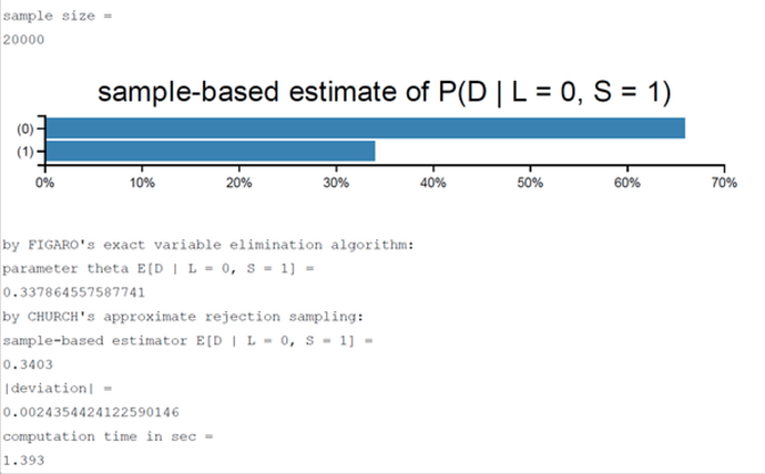
You mean, you would like to set evidence L = 0, and S = 1, and calculate posterior probabilities of other variables in the network P(D=1 | L = 0, S = 1)?
It could be done like this:

with pm.Model() as model:
    I_ = pm.Categorical('I', p=I)
    D_ = pm.Categorical('D', p=D)
    G_prob = T.shared(G)
    G_0 = G_prob[I_, D_]
    G_ = pm.Categorical('G', p=G_0)
    S_prob = T.shared(S)
    S_0 = S_prob[I_]
    S = pm.Categorical('S', p=S_0, observed = 1)
    L_prob = T.shared(L)
    L_0 = L_prob[G_]
    L_ = pm.Categorical('L', p=L_0, observed = 0)

So now you can do the inference like:

with model:
    trace = pm.sample(20000)

You’ve gotten your posteriors of D, I and G, and if you’d like make a querry for example:
P(D=1 | L = 0, S = 1):

If im not wrong, all you have to do is count how many times D was equal to 1 from all the samples…

Somebody correct me if i’m wrong (lucianopaz, junpenglao)

Or that could be just calculating posterior distribution, and if we wanted to evaluate quarry:

Since you already have samples from joint distribtuion given priors (or posteriors),
you can evaluate it as:

df = pm.trace_to_dataframe(trace)
P(D=1 | L = 0, S = 1) = P(D=1,L=0,S=1)/P(L=0,S=1) =
len(df_b = df.query(“L == 0 and S == 1 and G == 1”)/len(df_b = df.query(" S == 1 and G == 1")

lucianopaz · February 6, 2019, 11:10am

As @tomkov said, you can perform conditional sampling by setting some variables as observed. These variables will be fixed to 0 or 1 throughout the entire trace, so you cannot query values that are different from those. To get the probability of D=1 conditional on the observed L and S you can simply do np.mean(trace['D'] == 1)

tomkov · February 6, 2019, 12:39pm

to be honest, i’m not getting the right results with that method.
I’ve found somewhere on the Internet this example done with OpenBUGS:
This was thair network:

I’ve defined PCTs as:

D = np.array([0.6, 0.4])
I = np.array([0.7, 0.3])
G = np.array([[[0.3, 0.7],
               [0.05, 0.95]],
              [[0.9, 0.1],
               [0.5, 0.5]]])
S = np.array([[0.95, 0.05], 
              [0.2, 0.8]])
L = np.array([[0.1, 0.9], 
              [0.4, 0.6]])

On the other hand, with the code:

tomkov:

with pm.Model() as model:
    I_ = pm.Categorical('I', p=I)
    D_ = pm.Categorical('D', p=D)
    G_prob = T.shared(G)
    G_0 = G_prob[I_, D_]
    G_ = pm.Categorical('G', p=G_0)
    S_prob = T.shared(S)
    S_0 = S_prob[I_]
    S = pm.Categorical('S', p=S_0, observed = 1)
    L_prob = T.shared(L)
    L_0 = L_prob[G_]
    L_ = pm.Categorical('L', p=L_0, observed = 0)

and using

the result is: 0.53

rghelichi · February 6, 2019, 1:12pm

Thank you very much.
shouldn’t it give me the same answer as the query method @lucianopaz suggested?

rghelichi · February 6, 2019, 1:21pm

The example is taken from Koller’s book (Probabilistic graphical models Chapter 3)
The difference in your setup and her example is G has 3 and CPD of L is little bit different.

I tried using the posterior sampling using trace[‘D’] vs query method; I am getting the same answer with an error of third digit (0.601612 vs 0.603644)
Do you guys think there is an advantage of doing it through sampling with observed value vs using directly query method?

Thanks I truly appreciate your help saved me tons of time.

Ramin

tomkov · February 6, 2019, 3:04pm

I’ve tried both ways also, and compared them with Chpater 3, PGM Koller’s book.

The thing is, in case when you use query method, you’ve already made assumption the prior probabilities in you network are correct, and therefore you can get examples from joint distribution.

On the other hand, if you’re wrong about your priors (ex. change book probabilities to P(D=1)=0.01, and P(S=1)=0.001), then you’ll get better (and more correct) values if you’ve observed some evidence.

lucianopaz · February 6, 2019, 3:05pm

In your very particular case, I would favor what you call the query method. What truly underlies said method is that you draw single samples from the prior generative process and then you try to infer the probability of certain conditional outcomes. The query method works for this problem for three very important reasons:

The sample space of this problem is very small.
The inference is done based on the output of a single observed value, S=1 and L=0, and not a list of many iid observations that came from the generative process, if S and L's observed were longer arrays.
The event S=1 and L=0 is not highly unlikely, so drawing some scalar samples from the prior yields enough data to get a more or less precise answer.

When one of the previous three points does not hold, the query method stops being practical and one can only attempt to do MCMC.

On the other hand, when doing MCMC on discrete variables, we are forced to use metropolis Monte Carlo, and we must take more care that the chain converge, mix well, don’t get stuck and have low autocorrelation. If we don’t take these precautions, we end up with biased estimates. Usually NUTS is so efficient that if we don’t see divergences and the traces seem fine, we can work with all the points in the trace, but metropolis is much less efficient. It will likely be necessary to thin the chains to reduce the autocorrelations.

rghelichi · February 6, 2019, 4:41pm

Thank you very much for your kind help.

I agree. In case of changing the prior, the PJD I’ve gained with trace is not valid anymore and I have to resample the whole process again.

On the same note, I wonder if how I can estimate the prior (and more CPDs) better. Ideally, I would guess the prior should come from a Dirichlet distribution. I followed this example for the syntax:

Chris: Problem with pm.Categorical

import theano.tensor as tt
D = np.array([0.6, 0.4])
I = np.array([0.7, 0.3])
G = np.array([[[0.3, 0.4, 0.3],
[0.05, 0.25, 0.7]],
[[0.9, 0.08, 0.02],
[0.5, 0.3, 0.2]]])
S = np.array([[0.95, 0.05],
[0.2, 0.8]])
L = np.array([[0.1, 0.9],
[0.4, 0.6],
[0.99, 0.01]])
II = data.I.values # data = pm.trace_to_dataframe(prev_trace) from known priors
DD = data.D.values
GG = data.G.values
with pm.Model() as cpd_estimate:
Ie = pm.Dirichlet(‘Ie’, a = np.ones(2))
I_ = pm.Categorical(‘I’, p=Ie, observed=II)
De = pm.Dirichlet(‘De’, a = np.ones(2))
D_ = pm.Categorical(‘D’, p=De, observed=DD)
G_prob = pm.Dirichlet(‘Ge’, a=np.ones(G.shape), shape=G.shape)
G_0 = G_prob[I_, D_]
G_ = pm.Categorical(‘G’, p=G_0, observed=GG)
trace = pm.sample(1000)

it is very slow!!! (~2 draws/s) any suggestions? I can always use VI but I was wondering if there is something I could do to make it faster. It becomes really slow when I add G!

PS it seems there is something wrong about Dirichlet; the output of the trace log looks like this whenever I use Dirichlet in my model:

Sorry for these long messages. I really appreciate your help.

Ramin

rghelichi · February 6, 2019, 4:41pm

It makes total sense.

Thanks for the thorough explanation.

Ramin

tomkov · March 18, 2019, 1:09pm

Have you ever figured out why is it that slow?

rghelichi · April 12, 2019, 4:57pm

Hi,

Actually No, I believe better definition of the prior will lead to a faster sampling. and for now I use a very simple approach to approximate the priors better which works only for discrete variables.

Topic		Replies	Views
The pymc3 way: Linear regression and inferring given posterior/trace Questions	4	1755	May 9, 2018
Pymc3 likelihood math with non-theano function Questions theano	4	1070	September 25, 2017
Using theano scan with pymc3 Questions	3	864	December 4, 2020
Use xarray for traces Development	5	1730	June 15, 2017
PyMC3 Sampling with a model function that does not take array input natively v3 modeling	2	478	December 20, 2022

Making a query for a simple BN made in PYMC3

Related topics