Making predictions on model inputs based on observed outputs

I am fairly new to PyMC3 and I am trying to model the uncertainty propagation during the calibration process of a sensor. As such, the outputs of my model are [Y] and the inputs are [X]. xdata and ydata are the np.arrays containing my calibration data. My model looks` like this:

def volt_est(w,x):

return w[0] + w[1]*(1/x) + w[2]*(1/(x**2)) + w[3]*(1/(x**3)) + w[4]*(1/(x**4))

with pm.Model() as model:

sigma2_w = pm.Exponential('sigma2_w',lam=0.5, shape=5)
w = pm.Normal('w', mu=0, sigma=sigma2_w, shape=5)

# Input uncertanty

x = pm.Normal('x', mu=xdata, sigma=10., shape=xdata.shape[0], testval=xdata)

# Data Likelihood
x_like = pm.Normal('xdata', mu=x, sigma=0.0025, observed=xdata)
likelihood = pm.Normal('y', mu=volt_est(w,xdata), sigma=0.05, observed = ydata)

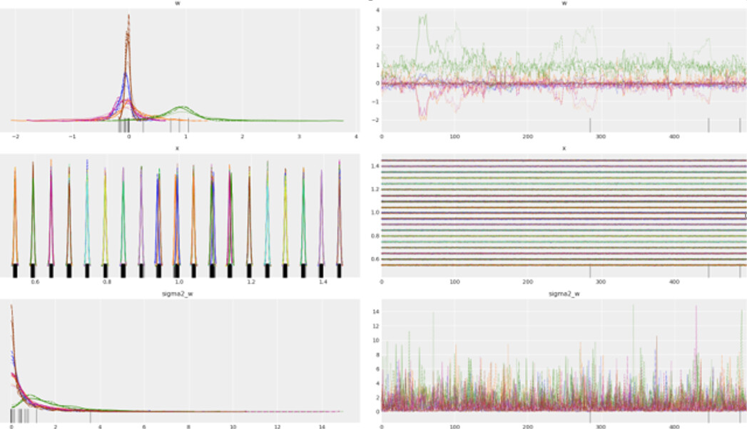
When I sample from the posterior I get the distributions for my weights ‘w’:

During an actual experiment, I am interested in retrieving an expectation and standard deviation for variable X based on a voltage input, Y. How can I do this?

I tried making X and Y shared variables, then setting the value of Y to my observed experiment value and finally, sample from the posterior to retrieve X but it did not work. Any thoughts?

Thank you!

Hi Santiago-

Looks to me like you’re calibrating a model in terms of P(Y|X) but then want to sample from P(X|Y). This is doable since the joint distribution P(X,Y) is what’s modeled, but sampling from a pre-image is not as straightforward as posterior prediction. I can think of two ways to do this.

Method 1: Keep your calibration data, and jointly calibrate P(Y_\mathrm{tr}|X_\mathrm{tr}) and sample P(X_{\mathrm{new}}|Y_{\mathrm{new}}). This would look like:

def ve(w, x):
    return w[0] + w[1]*(1/x) + w[2]*(1/(x**2)) + w[3]*(1/(x**3)) + w[4]*(1/(x**4))

with pm.Model() as mod:
    w_err = pm.Exponential('sig_w', lam=0.5, shape=5)
    w = pm.Normal('w', mu=0, sigma=w_err, shape=5)
    
    y = ve(w, x_train)
    lik = pm.Normal('y_lik', mu=y, sigma=y_err, observed=y_train)
    
    x_inf = pm.Bound(pm.Normal, lower=1e-3)('x_te', mu=np.mean(x_train), sigma=2, shape=3)
    y_inf = ve(w, x_inf)
    
    lik_yobs = pm.Normal('y_lik_te', mu=y_inf, sigma=y_err, observed=y_test[:3])
    
    tr = pm.sample(draws=1000, chains=6, cores=3, tune=1000, init='advi+adapt_diag')

from matplotlib import pyplot as mplt
plt = sbn.histplot(tr['x_te'], stat='count')
mplt.vlines(x=x_test[:3], ymin=0, ymax=7e3)

image

Problem: you’ve got to keep your data around every time you want to infer ‘x’, and the computation of a complicated likelihood can really slow down the sampling. An alternative is to extract (an approximation to) the posterior for w and use that alone:

w_mu = tr['w'].mean(axis=0)
w_sig = np.cov(tr['w'].T)

with pm.Model() as approx_post:
    w = pm.MvNormal('w', mu=w_mu, cov=w_sig, shape=(5,))
    x = pm.Bound(pm.Normal, lower=1e-3)('x', mu=np.mean(x_train), sigma=4)
    y = ve(w, x)
    y_lik = pm.Normal('y_lik', mu=y, sd=y_err, observed=y_test)
    
    tr2 = pm.sample(1000, chains=6, tune=1000, init='advi+adapt_diag')

plt = sbn.histplot(tr2['x'], stat='count')
mplt.vlines(x=x_test[:3], ymin=0, ymax=7e3)

image

You could also use the posterior of w (and the error variance y_err) outside of pymc3 to compute pre-images (be careful as your quartic may not be one-to-one):


def vei_np(w, x):
    # quartic in `x` rather than 1/x
    p = np.array([x ** i for i in range(5)])
    return np.dot(w, p)

def find_x(w, y):
    def obj(x):
        return (vei_np(w, x) - y)**2
    xinv = sp.optimize.minimize(obj, 1.).x[0]
    return 1/xinv

x_pre = np.array([[find_x(tr['w'][i,:], y + y_err * np.random.normal()) for y in y_test] for i in range(0,6000,5)])

plt = sbn.histplot(x_pre, stat='count')
mplt.vlines(x=x_test[:3], ymin=0, ymax=1210)

image

Hi Chris,

This is perfect, thanks. Since my calibration function is a one-to-one I ended up using your third recommendation because it was the fastest for me.

I would also recommend using a root finder (like sp.optimize.newton) since it’s much faster; the use of a least-squares minimization was just an illustrative hack.

1 Like