Hi everyone!
I am working on a model that should be dealing with gene expression data (so the real input to the model will be big). I am trying to fit some type of GLM model using the Negative Binomial (NB) distribution.
NB distribution has two parameters: \mu and \alpha. For now I assume only parameter \mu is a function of a time:=\mu = \mu(t), but later I want to extend it to the second parameter as well. I put a parametric form on \mu(t) = exp(b_{0} + b_{1} * f_1(t) + b_{2} * f_2(t) + \cdots). Where f_i(t) are precomputed quantities (they are radial basis functions here). I am trying to model each coefficient b_{i} using a separate Dirichlet process, so that genes that have similar patterns for example in terms of mean expression (this should be indicated by coefficient b_{0}) will fall into the same cluster. Think of this as I want to achieve an independent clustering for each regression coefficient.
The second parameter of the distribution, \alpha, is also modeled by a Dirichlet process.
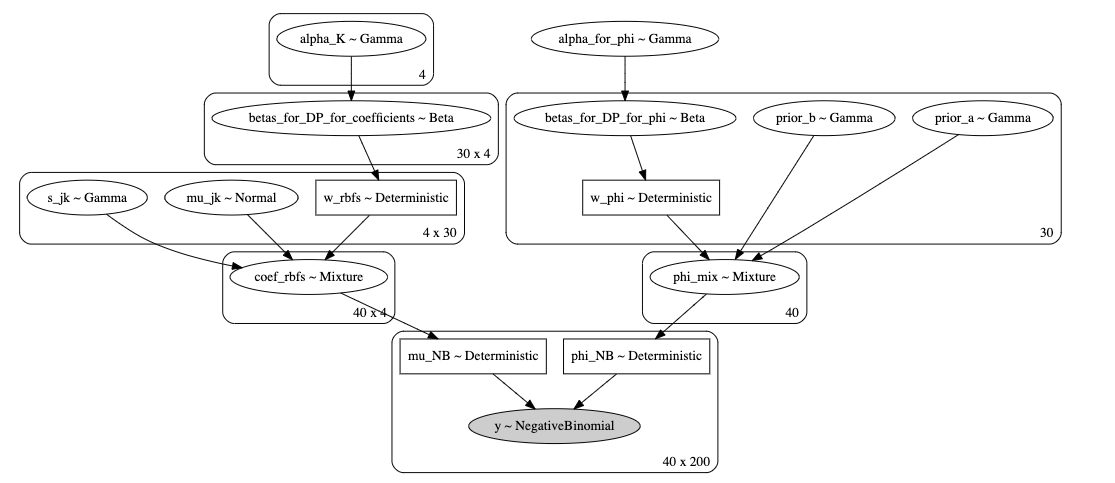
The graphical model is presented here:
I have N = 40 genes and P = 200 time points.
I sample 4 (an offset plus 3 RBFs) coefficients (b_{0} \cdots b_{3}) from Dirichlet processes 40 times (for each gene). I also sample \alpha 40 times for a separate Dirichlet process. Then I construct \mu(t) (denoted by mu_NB) and phi_NB = \alpha and pass it to the likelihood.
In my understanding this should work. In my toy example the full inference indeed works (the advi initialization fails though) but there are quite some number of divergences. The code for the model is presented below: K_mean is a number of RBFs plus offset: 4 here. J_mean:= number of components in each DP (30 here) for regression coefficients. J_phi:= number of components in DP for parameter \alpha (or phi as I call it here; 30 here as well).
### returns probabilities
def stick_breaking(v):
    cumprod = tt.extra_ops.cumprod(1. - v,axis=1)[:-1,:]
    ones    = tt.ones_like(v[:1,:])
    concat  = tt.concatenate([ones,cumprod],axis=0)
    breaks  = v * concat
    probs   = breaks/tt.sum(breaks,axis=0)
    return probs

### returns probabilities
def stick_breaking_for_array(beta):
    portion_remaining = tt.concatenate([[1], tt.extra_ops.cumprod(1 - beta)[:-1]])
    retVal = beta * portion_remaining
    retVal = retVal/tt.sum(retVal)
    return retVal
    # some starting points
    test_point_betas_for_DP = np.ones((J_mean,K_mean))*0.2
    testval_alpha_K         = np.ones((K_mean,))*3

with pm.Model() as model:
    ################################################## I. MU PART ################################

    ### prior for the concentraion : eq.8
    ### only mu (see likelihod) parameter is a linear combination of RBFs in this model (once I am sure it is working, it will be easy to extend for parameter phi)
    ### log_mu = b0*1 + b1 * f1 + b2* f2 + ...  (need not to forget to exponentiate later)
    ### we have K_mean (:= # of RBFs plus an offset) terms in the linear combination
    ### values (1, f1, f2, ...) come from Design Matrix which is computed above
    ### each coefficient b(i) (total # of coefficients is K_mean) comes from a Dirichlet Process
    ### we need K_mean independent concentration priors
    alpha_K           = pm.Gamma('alpha_K', 1., 1., shape = K_mean, testval = testval_alpha_K)


    ##### samples from beta (1,alpha) : eq.8
    ##### we need to sample J_mean (:= maximum number of clusters for a particular DP) samples for each of K_mean DP
    betas_for_mu      = pm.Beta('betas_for_DP_for_coefficients',
                                1.0,
                                alpha_K,
                                shape   = (J_mean,K_mean),
                                testval = test_point_betas_for_DP
                                )
    # stack of 4 independent 15-component weight arrays: in variable terms shape=(K_mean,J_mean)
    #w_mix_rbfs              = pm.Deterministic('w_for_mu',
    #                                            stick_breaking(betas_for_mu).T
    #                                          )

    ### eq.8 getting p(jk)
    w_mix_rbfs        = pm.Deterministic("w_rbfs",
                                         stick_breaking(betas_for_mu).T)


    #### now working with eq. 6,7
    #### define components: mu(jk) and s(jk)
    mu_jk  = pm.Normal("mu_jk",mu=0.0,tau=r_k,shape=(K_mean,J_mean))
    s_jk   = pm.Gamma("s_jk",alpha=1.0,beta=b_k,shape=(K_mean,J_mean))

    ####### still working with eq. 7
    ####### this is following the logic from: https://docs.pymc.io/api/distributions/mixture.html (about stacking the mixtures)
    # create a mixture and sample N times from it
    coef_rbfs               = pm.Mixture("coef_rbfs",w_mix_rbfs,
                                         comp_dists = pm.Normal.dist(mu=mu_jk,tau=s_jk,shape=(N,K_mean,J_mean)),
                                         shape = (N,K_mean)
                                        )
    ### create a linear combination and exponentiate it
    mu_NB                   = pm.Deterministic("mu_NB",
                                              tt.exp(tt.dot(coef_rbfs,DM_mean.T))
                                              )


    ################################################## II. PHI(ALPHA) PART ################################
    ### concentration prior for DP
    alpha_for_phi          = pm.Gamma('alpha_for_phi', 1., 1.,testval = 0.6)


    ### sample J_phi (:= number of possible components for parameter phi) values from beta distribution
    samples_from_beta_phi  = pm.Beta('betas_for_DP_for_phi',
                                      1.0,
                                      alpha_for_phi,
                                      shape   = J_phi,
                                      testval = 0.9
                                     )

    ### use stick-breaking function on samples from the previous step
    ### output is a weight array: all weights are from simplex
    w_phi                  = pm.Deterministic("w_phi",
                                              stick_breaking_for_array(samples_from_beta_phi))


    prior_a    = pm.Gamma('prior_a',1.0,1.0,shape = J_phi)
    prior_b    = pm.Gamma('prior_b',1.0,1.0,shape = J_phi)


    ### create a mixture for parameter phi -> sample N samples from a mixture
    phi_mix    = pm.Mixture('phi_mix',w_phi,
                            pm.Gamma.dist(prior_a,prior_b,shape=J_phi),
                            shape = N
                            )
    # expand
    phi_NB    = pm.Deterministic("phi_NB",
                                 (tt.ones([P,N]) * phi_mix).T)

    # likelihoood
    y          = pm.NegativeBinomial("y",
                                     mu       = mu_NB,
                                     alpha    = phi_NB,
                                     observed = samples)
I think it may be difficult to check this code without a context, so here is the link to the jupyter notebook: https://github.com/evgeniilobzaev/test_data/blob/master/the_only_working_copy.ipynb
The results of the toy input data are also there.
I am essentially trying to adapt the model from this paper (namely equations 6,7,8): https://arxiv.org/pdf/1904.11758.pdf to my needs.
Now the questions that I have:
- I am trying to construct the mixture model (variable coef_rbfs) as 4 stacked independent mixtures (I took inspiration from here: https://docs.pymc.io/api/distributions/mixture.html). Then I need to sample N=40 times from it. Did I do it correctly in terms of specifying the shapes or did I mess it up? The current specification does not complain but that is not a guarantee of the correct implementation.
- Why is there so many number of divergences? What can be the reason?
- Most importantly why VI does not work (I have some trials and checks suggested by pyMC3 community at the end of the jupyter notebook but they didn’t help) and what can be done to make it work? This is crucial, as for a true data where N can be 5000, full inference is infeasible.
Help would be very appreciated!
Evgenii