Dear Bayesians,
it might be of some help for some of you, today or later, to get an (up-to-date) installation protocol for GPU based sampling on Windows. I have seen some protocols based on pip here in the forum. However, I found that - hopefully - a purely conda based protocol seems to work.
First of all, make sure that the NVIDIA / CUDA drivers are installed properly by executing this on a PowerShell:
$ nvidia-smi
Sun Mar 16 09:18:12 2025
+-----------------------------------------------------------------------------------------+
| NVIDIA-SMI 572.70                 Driver Version: 572.70         CUDA Version: 12.8     |
|-----------------------------------------+------------------------+----------------------+
| GPU  Name                  Driver-Model | Bus-Id          Disp.A | Volatile Uncorr. ECC |
| Fan  Temp   Perf          Pwr:Usage/Cap |           Memory-Usage | GPU-Util  Compute M. |
|                                         |                        |               MIG M. |
|=========================================+========================+======================|
|   0  NVIDIA GeForce RTX 5070 Ti   WDDM  |   00000000:01:00.0  On |                  N/A |
|  0%   53C    P5             21W /  300W |   15663MiB /  16303MiB |      0%      Default |
|                                         |                        |                  N/A |
+-----------------------------------------+------------------------+----------------------+
This was all pre-installed by my PC vendor, therefore I did not have to do anything.
Next, it is still - unfortunately - not possible to install the relevant libraries directly in a Windows Python environment. This means, you need to use a WSL / Ubuntu based Python.
To install WSL, do this in a PowerShell:
wsl --install
After installation, look which Ubuntu is available:
wsl --list --online
I made a decision for:
wsl --install -d Ubuntu-22.04
After installation, open the “Terminal” app and create a new tab with your Ubuntu running. The next step is to install a Conda based Python installation in this Ubuntu. I did this by the following steps:
wget https://repo.anaconda.com/miniconda/Miniconda3-latest-Linux-x86_64.sh
bash Miniconda3-latest-Linux-x86_64.sh
source ~/.bashrc
Make conda-forge available:
conda config --add channels conda-forge
conda config --set channel_priority strict
You can now create a new conda environment for your pymc stuff. As I had some trouble with Python 3.12, I finally used a 3.11 environment:
conda create -n jax-env python=3.11
conda activate jax-env
Install mamba to get things done faster:
conda install -n base -c conda-forge mamba
Now install the relevant libraries:
mamba install -c conda-forge pymc bambi arviz nutpie blackjax numpyro
And some additional stuff
mamba install -c conda-forge matplotlib seaborn scikit-learn gputil jupyter
The environment is now created. To use it in a Jupyter Notebook in a Windows IDE, you have to configure this as your runtime. I am using DataSpell from Jetbrains, and I guess the configuration would be similar in IntelliJ or PyCharm. However, I do not know how this would work in VS Code.
In your project configuration, you add a new interpreter and choose “On WSL”:

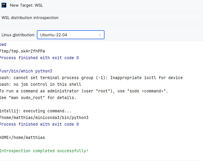
In the following dialog, you choose your installed Ubuntu:
In the following dialog, you choose “Conda environment” and you should find your configured environment in the dropdown:

After creation, you should find this interpreter in the list and can choose it for your project.

To use this interpreter for a Jupyter notebook, you can configure it as a “Managed Server”:

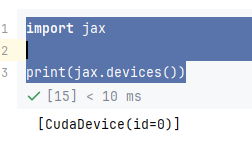
Now check some versions:


And here are some sampling times with a very simple model. I assume that GPU is not the right mode for a model with only one observed variable, because GPU will only pay out for much more dimensions. Or did I something wrong with the configuration?
true_mean_of_generating_process = 5
true_sigma_of_generating_process = 2

observed_data = np.random.normal(loc=true_mean_of_generating_process,
                                 scale=true_sigma_of_generating_process,
                                 size=100)

with pm.Model() as model_mean:
    mu = pm.Normal("mu", mu=0, sigma=10)
    sigma = pm.HalfNormal("sigma", sigma=10)

    likelihood = pm.Normal("likelihood",
                           mu=mu,
                           sigma=sigma,
                           observed=observed_data)

    # CPU
    # runtime: 3.28 seconds (AMD Ryzen 9 9900X)
    # idata_mean_cpu = pm.sample(
    #     draws=8000,
    #     tune=1000,
    #     chains=4,
    #     progressbar=False)

    # GPU with numpyro
    # runtime: 1m 49 seconds
    # idata_mean_numpyro = pm.sample(
    #     draws=8000,
    #     tune=1000,
    #     chains=4,
    #     progressbar=False,
    #     nuts_sampler="numpyro")

    # GPU with blackjax
    # needs the argument "chain_method" : "vectorized" to run without error
    # runtime: 20 seconds
    # idata_mean_blackjax = pm.sample(
    #     draws=8000,
    #     tune=1000,
    #     chains=4,
    #     progressbar=False,
    #     nuts_sampler="blackjax",
    #     nuts_sampler_kwargs={"chain_method" : "vectorized"})

    # GPU with nutpie
    # runtime: 1m 31 seconds
    # idata_mean_nutpie = pm.sample(
    #     draws=8000,
    #     tune=1000,
    #     chains=4,
    #     progressbar=False,
    #     nuts_sampler="nutpie",
    #     nuts_sampler_kwargs={"backend" : "jax"})
Best regards
Matthias