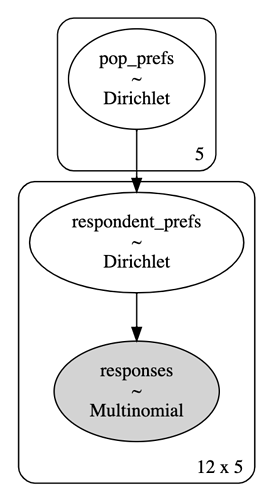
(newbie) using Dirichlet for partial pooling for likert-like survey responses

I am trying to use an HGLM to model responses to a preference test. Each survey question shows the user two versions of the same image: one filtered by algorithm A v.s. one filtered by algorithm B. The possible responses are:

  • Strongly Prefer A
  • Prefer A
  • No Preference
  • Prefer B
  • Strongly Prefer B

… except users aren’t actually told which is A or B.

I am trying to create a model that will, to the extent possible, characterise the preferences of all people, not just those who responded. It must be resilient to different people answering a different number of questions.

Here’s my code, and some data from my trial survey…

# Data from survey respondents.
df = pd.DataFrame(
    columns = ['STRONG_A', 'A', 'NO_PREF', 'B','STRONG_B'],
    data = [
        [14,  7,   4,  11,  42],
        [3,   2,   0,   4,  13],
        [1,   3,  16,  17,  15],
        [2,   4,   5,  14,   7],
        [1,   5,   2,   7,  20], 
        [7,   1,   1,   7,  14],
        [5,   9,  16,  10,  26],
        [9,   0,   7,  12,  22],
        [6,   2,   1,   4,  28],
        [0,   2,   8,  11,  10],
        [0,  10,   3,  11,  26],
        [1,  10,   5,  22,  20],
    ],
)
# Number of responses from each person.
df_n = df['STRONG_A'] + df['A'] + df['NO_PREF'] + df['B'] + df['STRONG_B']

n_options = 5
n_respondents = len(df)
with pm.Model() as model:
    # The preferences of all people, not just those who responded.
    pop_prefs = pm.Dirichlet(
        "pop_prefs",
        a=np.ones(n_options),
        shape=n_options,
    );
    # The preferences of each survey respondent.
    respondent_prefs = pm.Dirichlet(
        "respondent_prefs",
        a=pop_prefs,
        shape=(n_respondents, n_options),
    );
    responses = pm.Multinomial(
        "responses", 
        n=df_n, 
        p=respondent_prefs, 
        shape=(n_respondents,n_options),
        observed=df
    )
    
    trace = pm.sample(
        10000,
        tune=5000,
        return_inferencedata=True
    )
    az.plot_trace(trace)

az.summary(trace, var_names=["pop_prefs"])

Here are the results…


My expectation was that pop_prefs would characterise the preferences of the population, whilst respondent_prefs would account for variation from the “typical” person (loosely speaking). Running the model gave an expected probability of responding STRONGLY_PREFER_B of 0.264. If we take the average from the raw data, it’s .446. At first I assumed the discrepancy was due to regularization from a flat prior, but if I copy paste the data three times to simulate having more evidence, the result remains the same except with a narrower confidence interval, which suggests I’m misunderstanding something. The same happens with synthetic data generated from a distribution.

What am I doing wrong? I’m just an engineer who is trying to teach themselves Bayesian modelling, and I would greatly appreciate any guidance. I’ve read Statistical Rethinking twice now :sweat_smile: Thank you!

2 Likes

The large number of divergences implies that you should ignore the posterior you are currently getting. I increased the number of tuning samples and the target acceptance rate and that eliminated the divergences.

trace = pm.sample(tune=2000, target_accept=.9)

However, it doesn’t change the estimates much.

If you inspect the summary of respondent_prefs, you should see that they are pretty close to the individual rows of your data. But the hyperparameter pop_prefs are not close to the grand averages as you note. You are correct that pop_prefs characterizes the preferences of the population, but does not reflect the grand means. Why? Because each individual respondent doesn’t respond in way consistently reproduces the population means (i.e., you have heterogeneity within your sample). Imagine we have only 2 respondents. If one respondent only produces STRONGLY_PREFER_A responses and a second respondent only produces STRONGLY_PREFER_B responses, what should we expect the posterior of the hyperparameter to be? Half the responses we see are STRONGLY_PREFER_A. However, half of our respondents produced it with probability 1.0 and half of them produced it with probability 0.0. So we should be very uncertain about the population-level population of having a STRONGLY_PREFER_A tendency. Specifically, we should not be convinced that the population parameter associated with a STRONGLY_PREFER_A response is definitely near 0.5. To confirm this, you can look at the full posterior rather than the means produced by az.summary(). Specifically, you can call:

az.plot_posterior(trace, var_names=["pop_prefs"])

Which shows a posterior that seems consistent with a large degree of uncertainty about the population (hyper)parameters:

This is also why duplicating your data many times doesn’t change things much at the population level. The heterogeneity among your respondents is roughly the same when you simply cut and paste your 12 respondents over and over.

2 Likes

I think there might be confusion because the hyperparameter pop_prefs are over the concentration parameter of the Dirichlet prior. I could be mistaken, but I don’t think a concentration parameter \alpha_i gives the percentage share of draws from the distribution that will be of class i (although it might be possible to recover this percentage with some algebra). Furthermore, the Dirichlet alphas aren’t bounded between 0-1, so I don’t know if modeling them as coming from a Dirichlet makes sense.

I tried running your model again, using a hierarchical normal prior over the multinomial probability, which I then put into a softmax to ensure everything added up to 1 row-wise. I figure this will make everything easier to interpret, because we only have to reason about the softmax, and not about the Dirichlet distribution.

options_idx, options = pd.factorize(df.columns)
respondents_idx, respondent = pd.factorize(df.index)
n_respondents, n_options = df.shape

coords = {'options':options, 'respondents':respondents}

with pm.Model(coords=coords) as model:
    pop_mu = pm.Normal('pop_mu', mu=0.0, sigma=1.0, dims=['options'])
    pop_sigma = pm.HalfCauchy('pop_sigma', beta=0.8, dims=['options'])
    respondent_offset = pm.Normal('respondent_offset', mu=0.0, sigma=1.0, dims=['respondents', 'options'])
    respondent_prefs = pm.Deterministic('respondent_prefs', pop_mu + pop_sigma * respondent_offset, dims=['respondents', 'options'])
    
    responses = pm.Multinomial(
        "responses", 
        n=df_n.values, 
        p=pm.math.softmax(respondent_prefs, axis=1), 
        dims=['respondents', 'options'],
        observed=df
    )
    
    prior = pm.sample_prior_predictive()

This sampled without divergences (with adapt_diag_grad and target_accept=0.9), although so did your original model (with default settings) when I tried it, so idk. Anyway, I get the following estimates for the population averages:

                   mean     sd  hdi_3%  hdi_97%  mcse_mean  mcse_sd  ess_bulk  ess_tail  r_hat
pop_mu[STRONG_A] -0.759  0.544  -1.794    0.242      0.020    0.014     722.0    1501.0   1.00
pop_mu[A]        -0.486  0.483  -1.378    0.419      0.020    0.014     599.0    1250.0   1.00
pop_mu[NO_PREF]  -0.427  0.501  -1.354    0.520      0.019    0.013     693.0    1244.0   1.01
pop_mu[B]         0.428  0.462  -0.411    1.304      0.019    0.013     611.0    1121.0   1.01
pop_mu[STRONG_B]  1.048  0.469   0.182    1.943      0.019    0.014     585.0    1164.0   1.00

To recover estimated population proportions, I put the means into a softmax and compare with the data:

print((df.mean() / df.mean().sum())
     .to_frame()
     .rename(columns={0:'data_proportion'})
     .assign(estimated_proportion = softmax(az.summary(trace, var_names=['pop_mu'])['mean']).values)
     .to_string())

Which gives:

          data_proportion  estimated_proportion
STRONG_A         0.089908              0.076470
A                0.100917              0.100474
NO_PREF          0.124771              0.106580
B                0.238532              0.250610
STRONG_B         0.445872              0.465866

These seem reasonable, so I feel like it’s on the right track. Again, there might be a way to do it by interpreting the Dirichlet concentrations, but I would need to hit the books to figure it out.

3 Likes

Shows how closely I looked at the model (i.e., not very). Yeah, using draws from a Dirichlet as the concentrations in a second Dirchlet (or set of Dirchlets) probably isn’t what you want!

1 Like

Thank you! This has been extremely helpful!


A note for anyone who may stumble upon this in future…

For whatever reason, pm.math.softmax didn’t exist for me. However Jesse’s solution with these two small changes gave the same result…

    responses = pm.Multinomial(
        "responses", 
        n=df_n.values, 
        # p=pm.math.softmax(respondent_prefs, axis=1),
        p=theano.tensor.nnet.softmax(respondent_prefs),  # <---- Replacement
        shape=(n_respondents,n_options),
        observed=df
    )

and

def softmax(x):
    e_x = np.exp(x - np.max(x))
    return e_x / e_x.sum()

print(softmax(az.summary(trace, var_names=['pop_mu'])['mean']))
2 Likes

Ah yeah sorry i cut off where i imported scipy.special.softmax for the post-processing.

You don’t have pm.math.softmax because it looks like you’re running PyMC3. I ran mine with PyMC 4.0.

1 Like