Poisson regression model for beginner

Hi evertone from the comunity.

I am a beginner on data analysis in general and I have this project to do and I hope someone could give me some advice.
The project consists of modelling counting data with a Poisson regression model and make point estimate the paramaters of the model using Metropolis-Hastings algorithm using pymc3 library.
The dataset that I have to use is a very simple one. It’s about observations of Insurance Motor Third Party Claims (both frequenct and severity). I’ll link the full description of the dataset below.

https://search.r-project.org/CRAN/refmans/GLMsData/html/motorins.html

There are two issues that I am dealing with:

  1. Do I have to do some preprocessing step before running the algorithm? If so, how do I do it?

  2. I built a model following the Poisson regression model in the example section, but still the the algorithm is too slow. How I can improve performance?
    Here is the code I used until now:

import arviz as az
import bambi as bmb
import matplotlib.pyplot as plt
import numpy as np
import pandas as pd
import pymc3 as pm
import seaborn as sns
import theano
import theano.tensor as tt
import xarray as xr

from formulae import design_matrices

print(f"Running on PyMC3 v{pm.__version__}")
print(f"Running on Arviz v{az.__version__}")

df = pd.read_csv('SwedishMotorInsurance.csv')
df.head()

df['Rate']=df['Claims']/df['Insured']

fml = "linear ~ Kilometres + Zone + Bonus + Make"

df_1=df[['linear','Kilometres','Zone','Bonus','Make']]

dm = design_matrices(fml, df_1, na_action="error")

mx_ex = dm.common.as_dataframe()
mx_en = dm.response.as_dataframe()

with pm.Model() as model:

    # define priors, weakly informative Normal
    b0 = pm.Normal("Intercept", mu=0, sigma=10)
    b1 = pm.Normal("Kilometres", mu=0, sigma=10)
    b2 = pm.Normal("Zone", mu=0, sigma=10)
    b3 = pm.Normal("Bonus", mu=0, sigma=10)
    b4 = pm.Normal("Make", mu=0, sigma=10)
    

    # define linear model and exp link function
    theta = (
        b0
        + b1 * mx_ex["Kilometres"].values
        + b2 * mx_ex["Zone"].values
        + b3 * mx_ex["Bonus"].values
        + b4 * mx_ex["Make"].values
    )

    ## Define Poisson likelihood
    y = pm.Poisson("y", mu=tt.exp(theta), observed=mx_en["linear"].values)
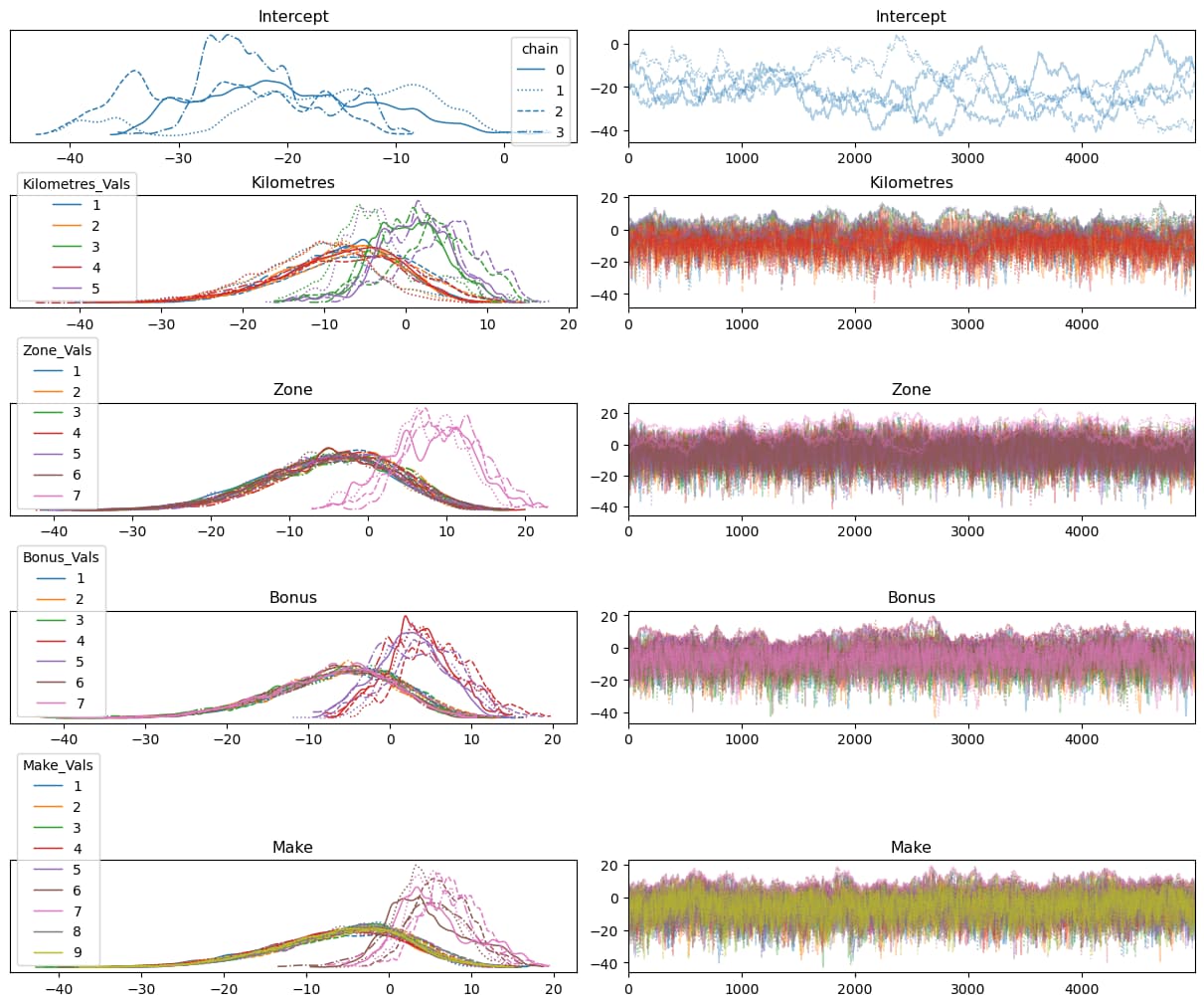
with model:
    trace = pm.sample(draws=5000, tune=500, cores=4, random_seed=45, step=pm.Metropolis())
    
pm.summary(trace)

How would you modify it?

Here is the dataset file.
SwedishMotorInsurance.csv (49.6 KB)

Hope this would be useful for other beginners like me.

I’m also new to PYMC, but have been trying to model with the related Negative Binomial Distribution, and similarly with categorical independent values. I’ve had trouble finding much documentation on distribution indexing, but have pieced together some code through other posts, so I adapted some of my code to your model. It generates an equivalent model as best as I can tell, and samples in under 2 minutes for me.


Imports

import arviz as az
import matplotlib.pyplot as plt
import pymc as pm
import pandas as pd
from pandas.api.types import CategoricalDtype

Preprocessing

print(f"Running on PyMC3 v{pm.__version__}")
print(f"Running on Arviz v{az.__version__}")

df = pd.read_csv('data/SwedishMotorInsurance.csv')
# making Pandas Categorical. You could add Names to the numerical codes if you wish
df['Kilometres'] = df['Kilometres'].astype(CategoricalDtype())
df['Zone'] = df['Zone'].astype(CategoricalDtype())
df['Bonus'] = df['Bonus'].astype(CategoricalDtype())
df['Make'] = df['Make'].astype(CategoricalDtype())

df['Rate']=df['Claims']/df['Insured']

df.head()

Model

COORDS = {'Kilometres_Vals':df['Kilometres'].cat.categories.values, 
          'Zone_Vals':df['Zone'].cat.categories.values, 
          'Bonus_Vals':df['Bonus'].cat.categories.values, 
          'Make_Vals':df['Make'].cat.categories.values,
          "obs_idx": df.index}

with pm.Model(coords=COORDS) as model:

    # define priors, weakly informative Normal
    b0 = pm.Normal("Intercept", mu=0, sigma=10)
    b1 = pm.Normal("Kilometres", mu=0, sigma=10, dims="Kilometres_Vals")
    b2 = pm.Normal("Zone", mu=0, sigma=10, dims="Zone_Vals")
    b3 = pm.Normal("Bonus", mu=0, sigma=10, dims="Bonus_Vals")
    b4 = pm.Normal("Make", mu=0, sigma=10, dims="Make_Vals")

    km_data = pm.ConstantData('Kilometres_data', df['Kilometres'].cat.codes.to_numpy(), dims="obs_idx")
    zone_data = pm.ConstantData('Zone_data', df['Zone'].cat.codes.to_numpy(), dims="obs_idx")
    bonus_data = pm.ConstantData('Bonus_data', df['Bonus'].cat.codes.to_numpy(), dims="obs_idx")
    make_data = pm.ConstantData('Make_data', df['Make'].cat.codes.to_numpy(), dims="obs_idx")

    # not making this a Deterministic because it would take the dims of # of datapoints
    theta = b0 + b1[km_data] + b2[zone_data] + b3[bonus_data] + b4[make_data]

    # ## Define Poisson likelihood
    y = pm.Poisson("y", mu=pm.math.exp(theta), observed=df['Rate'].values)

pm.model_to_graphviz(model)

Sample

with model:
    trace = pm.sample(draws=5000, tune=500, cores=4, random_seed=45, step=pm.Metropolis())
    
pm.summary(trace)

100.00% [22000/22000 01:50<00:00 Sampling 4 chains, 0 divergences]
Sampling 4 chains for 500 tune and 5_000 draw iterations (2_000 + 20_000 draws total) took 110 seconds.

|mean|sd|hdi_3%|hdi_97%|mcse_mean|mcse_sd|ess_bulk|ess_tail|r_hat|
|Intercept|-21.138|8.832|-38.752|-5.647|2.836|2.069|10.0|40.0|1.31|
|Kilometres[1]|-8.326|7.546|-22.524|5.354|1.062|0.755|49.0|352.0|1.06|
|Kilometres[2]|-8.384|7.528|-22.646|5.808|0.996|0.708|54.0|321.0|1.05|
|Kilometres[3]|0.082|5.562|-10.302|10.515|1.475|1.065|15.0|65.0|1.20|
|Kilometres[4]|-8.937|7.757|-23.532|5.206|0.691|0.490|97.0|423.0|1.04|
|Kilometres[5]|1.182|5.566|-8.483|11.945|1.522|1.100|14.0|54.0|1.22|
|Zone[1]|-5.257|8.245|-21.075|9.332|0.287|0.203|760.0|1336.0|1.01|
|Zone[2]|-4.591|8.190|-19.726|10.162|0.291|0.206|707.0|931.0|1.01|
|Zone[3]|-4.900|8.247|-20.375|10.100|0.311|0.220|621.0|1090.0|1.01|
|Zone[4]|-4.683|8.157|-20.335|9.482|0.408|0.288|377.0|828.0|1.02|
|Zone[5]|-5.012|8.275|-21.077|9.448|0.327|0.232|583.0|1014.0|1.01|
|Zone[6]|-4.879|8.370|-20.631|10.338|0.327|0.232|585.0|1063.0|1.01|
|Zone[7]|8.438|5.107|-1.407|17.877|0.900|0.642|32.0|113.0|1.08|
|Bonus[1]|-6.244|7.774|-21.171|7.367|0.273|0.193|743.0|1166.0|1.01|
|Bonus[2]|-6.905|7.864|-21.760|7.405|0.278|0.197|718.0|853.0|1.01|
|Bonus[3]|-6.822|7.791|-21.670|6.898|0.331|0.234|495.0|1052.0|1.01|
|Bonus[4]|4.317|4.472|-3.805|12.705|0.560|0.398|61.0|185.0|1.07|
|Bonus[5]|3.225|4.568|-5.171|11.791|0.569|0.404|63.0|194.0|1.07|
|Bonus[6]|-6.820|7.575|-21.056|6.621|0.321|0.227|493.0|834.0|1.01|
|Bonus[7]|-7.098|7.639|-21.793|6.213|0.310|0.220|548.0|905.0|1.02|
|Make[1]|-5.948|8.054|-21.779|8.020|0.312|0.221|628.0|766.0|1.00|
|Make[2]|-5.653|7.975|-21.086|8.439|0.316|0.223|582.0|892.0|1.01|
|Make[3]|-5.326|8.008|-20.667|8.656|0.270|0.191|815.0|1060.0|1.00|
|Make[4]|-6.222|8.060|-21.833|7.777|0.321|0.227|561.0|839.0|1.01|
|Make[5]|-5.364|7.761|-20.000|8.180|0.215|0.152|1116.0|1702.0|1.01|
|Make[6]|5.070|4.270|-2.444|13.567|0.464|0.329|85.0|162.0|1.04|
|Make[7]|6.183|4.122|-0.865|14.679|0.457|0.324|81.0|141.0|1.04|
|Make[8]|-5.438|7.866|-20.660|8.451|0.323|0.228|520.0|862.0|1.01|
|Make[9]|-5.686|7.940|-21.525|7.588|0.292|0.206|623.0|851.0|1.01|

Plot Trace

az.plot_trace(
    trace,
    backend_kwargs={"layout": "constrained"}, legend=True
);


I hope this helps. Also, if any more advanced users can improve upon it, that would help my own modeling as well. Also, if anyone knows where the actual documentation is on indexing.
e.g. b1[km_data] or b1[km_data, zone_data]
I’m particualarly interested in generalizing to higher dimensional distributions.

Hi @Riccardo_Zhu!

Looking at your model there are a few things that spring to mind:

  1. Its not clear what you are trying to predict here. The linear term in your model specification isn’t in the original dataset or created in your code. I am going to take it as a given you want to predict the number of claims, because in the linked page to the data it says ‘…For this data, the number of claims has a Poisson distribution’. So I am going to assume that’s what you’re after. You could aim to predict Rate, but a Poisson likelihood would probably not the best for that. If thats what you want, we can lean on the Binomial and discuss further.

  2. Do you have to use pm.Metropolis as the step? The default NUTS is state-of-the-art.

  3. Part of the reason the model sampled so slowly to begin with is because of the variable specification. Reading the linked document it looked like all variables in the equation apart from bonus were categorical, while the original approach assumed they were continuous. You can have formulae force them to categories as I do below, or use pd.Categorical to assign categorical versions. The model will then have ‘dummy’ coefficients contrasting each category with the reference.

My version of your model is below, sampling in about 30-40 seconds (I am using PyMC 5.5, and suggest you upgrade if you can!). I’ve used Metropolis as the step but I do get convergence warnings, but none with NUTS:

df = pd.read_csv('SwedishMotorInsurance.csv')

# Create the design matrix using formulae
# Wrapping the variable in 'C()' enforces categorical values, with the first entry as the reference
dm = design_matrices('Claims ~ C(Kilometres) + C(Zone) + Bonus + C(Make)', data=df, na_action='error')

# Expand out into X (ex) and y (en)
X = dm.common.as_dataframe()
y = dm.response.as_dataframe().squeeze() # This ensures y is 1-dimensional. 2D observed values cause issues for sampling as the model assumes it needs to predict for multiple observed responses.

# Create labelled coords which help the model keep track of everything
c = {'predictors': X.columns, # Model now aware of number of and labels of predictors
     'N': range(len(y))} # and number of observations

# Set up the model
with pm.Model(coords=c) as poisson_reg:
    
    # Set the data (if you want to), and convert to NumPy arrays
    Xdata = pm.MutableData('Xdata', X.to_numpy())
    Ydata = pm.MutableData('Ydata', y.to_numpy())
    
    # You use the same priors for each coefficient in the model, so this can be specified like this
    # If you wish to use different priors you must do so like in your original parameterisation
    beta = pm.Normal('beta', mu=0, sigma=10, dims='predictors')
    
    # Can now take the linear combination of Xdata with beta, and exponent it - Xdata contains the Intercept column so this is no problem
    theta = pm.math.exp(Xdata @ beta) # @ operator is for matrix multiplication 
    
    # Plug into the Poisson likelihood
    pm.Poisson('y', mu=theta, observed=Ydata)
    
    # Sample according to your specifications, but tune for longer and take fewer draws
    trace = pm.sample(draws=1000, tune=3000, cores=4, random_seed=45, step=pm.Metropolis())

I do get some bad r-hat values from this which is problematic, but these do go away with the use of NUTS. The model sampling now comes at a cost - now we have the issue of interpreting the categorical coefficients for variables like Kilometres, which represent the difference in the rate of the observed counts. So for example in my output, the coefficient of Zone 5 is -1.358. exp(-1.358) ~ 0.25, so changing from Zone 1 to Zone 5, the rate of claim counts will change by a factor of 0.25, assuming all other values in the regression are held constant (beware of the fact this implies zero bonus make == 1 and kilometres == 1). Hope that helps!

@GrantDaly does the categorical predictor approach help your model parameterisation too?

Thank you @alj for you answer!

Yes, want I want to predict is the number of Claims. I’m sorry if it was not clear on my code. I tried different solution, that’s why I computed a new variable rates.

I know the default sampling method is NUTS. Using Metropolis is the specific of my own project. The topic is indeed Metropolis-Hastings Algorithm.

I tried copy and paste your code on my notebook, but when I run the code there are a lot of overflow during computation. I think it’s due to the fact that there are lots of zeros in the dataset in ‘Claims’ variable. Do I have to add some code before the “pm.Model” part?

Those overflows don’t seem to appear with NUTS so I wouldn’t like to comment on what’s causing them (though I can definitely see them too using Metropolis) - probably better for some of the devs to weigh in on this stuff, sorry!

Looks like there’s about 17% zeros in claims which may be enough to warrant the ZeroInflatedPoisson as the likelihood. That’s easy enough to implement, and you can compare the two models via az.compare to see which has better predictive ability. Looking at the spread of counts though you may want to try a Negative Binomial too.

I hope that helps!

The exponential function is prone to overflow if the scale of the input features are “large”. It’s good practice to always standardize (subtract mean, divide by std) all inputs and targets before you run a GLM. I believe Bambi does this for you automatically. See this discussion, for example. MH probably overflows more than NUTS because, prior to scale tuning, the sampler is drunkenly taking large steps into idiotic regions of the parameter space where theta ends up being too big.

2 Likes