I have a problem getting the posterior distributions of the learned parameters in a Bayesian hierarchical model lining up with their expected values from the data.
A description of the set up is as follows:
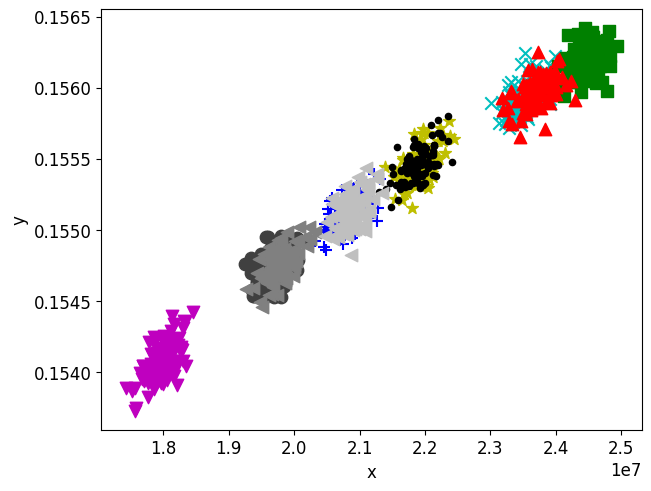
I have a dataset of x and y value pairs, as plotted below. Each of the five groups belongs to an individual population member, k, such that there are 1:K members where K=10. Each population member has 100 observations.
This dataset has been generated using numpy normal distributions in the following way:
import numpy as np
import matplotlib.pyplot as plt
import pymc as pm
import arviz as az

def surrogate(x):
    y = (2.9208426988769278e-40*(x**5)) - (5.186085828407714e-32*(x**4)) + (3.6864750447769966e-24*(x**3)) - (1.3448985532835548e-16*(x**2)) + (2.7318885815746297e-09*x) + 0.1318751022737149
    return y

# Keep it reproducable
np.random.seed(0)

##### Generate data Y
# set up our data
K = 10 # number of population members
N = 100 # number of observations

data_description = "_"+ str(K) + "K_" + str(N) + "N"

# # True global parameters (these will need priors on in the inference). We use these to draw local parameters
GEk = [20e6, 2e6]  # true expectation
GVk = [2e5, 1e4] # true variance

# Draw K local means
LEk = np.random.normal(GEk[0], GEk[1], size=K)
# Draw K local variances
LVk = np.random.normal(GVk[0], GVk[1], size=K)


# ---- draw stiffness realisations for each turbine (balanced dataset)
k = []
turbines = []
for i in range(K):
    k.append(np.random.normal(LEk[i], LVk[i], size=N)) # size T
    for j in range(N):
        turbines.append(i)
k = np.array(k).flatten()
turbines = np.array(turbines).flatten()

sigma_true = 0.0001  # measurement noise


# Create true data
measurement_noise = np.random.normal(0, sigma_true, size=N*K)

data = measurement_noise + surrogate_model # add some gaussian noise to the data, scaled by sigma


np.savetxt("data" + data_description + ".csv", data, delimiter=",") # save
np.savetxt("LEk" + data_description + ".csv", LEk, delimiter=",") # save
np.savetxt("LVk" + data_description + ".csv", LVk, delimiter=",")
np.savetxt("k" + data_description + ".csv", k, delimiter=",") # save
np.savetxt("turbines" + data_description + ".csv", turbines, delimiter=",") # save
np.savetxt("x_true" + data_description + ".csv", x_true, delimiter=",") # save
I have then tried to create a partially pooled model with PyMC, where I place hyperpriors over the global parameters which feed into the prior for the individual realisations of the x values. y values are then created with mean being the value of the surrogate function, with standard deviation (sigma) being the noise added to this function.
data_description = "_10T_100N"
wn_true = np.genfromtxt('data' + data_description + '.csv', delimiter=',')
k_true = np.genfromtxt('k' + data_description + '.csv', delimiter=',')
turbines = np.genfromtxt('turbines' + data_description + '.csv', delimiter=',')
turbines = turbines.astype(int)
LEk = np.genfromtxt('LEk' + data_description + '.csv', delimiter=',')
LVk = np.genfromtxt('LVk' + data_description + '.csv', delimiter=',')
K=int(len(LEk))
N=int(len(k_true)/K)
### Partially pooled (untransformed)
def surrogate(x):
y = (2.9208426988769278e-40*(x**5)) - (5.186085828407714e-32*(x**4)) + (3.6864750447769966e-24*(x**3)) - (1.3448985532835548e-16*(x**2)) + (2.7318885815746297e-09*x) + 0.1318751022737149
return y
print(f"Running on PyMC v{pm.__version__}")
with pm.Model() as hierarchical_model:
# priors
GEk = pm.Gamma("GEk", mu=25e6, sigma=5e6) # hyperprior 1
GVk = pm.Gamma("GVk", mu=8e4, sigma=1e5) # hyperprior 2
k = pm.Normal('k', mu=GEk, sigma=GVk, shape=K)
# measurement noise
gamma = pm.Uniform("gamma", lower=0, upper=0.001)
obs = pm.Normal('obs', mu=surrogate(k[turbines]), sigma=gamma, observed=wn_true)
hierarchical_trace = pm.sample(return_inferencedata=True, chains=4, tune=2000, draws=2000)
plt.rcParams['figure.constrained_layout.use'] = True
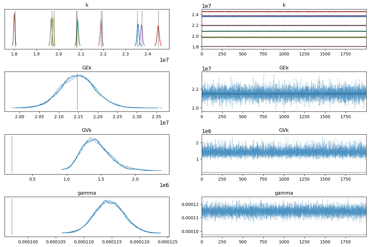
az.plot_trace(hierarchical_trace, lines=[("GEk", {}, np.mean(LEk)), ("GVk", {}, np.mean(LVk)), ("k", {}, LEk), ("gamma", {}, np.std(wn_true - surrogate(k_true)))])
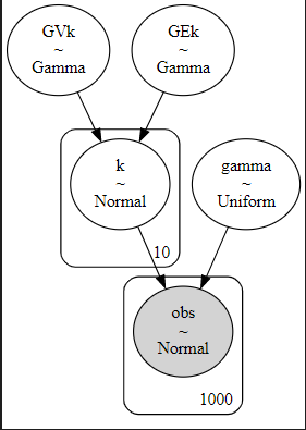
For further clarity, the model looks like this:
Observations:
- the mode of the population standard deviation is much too high compared to the expected value (shown by the vertical black lines)
- sig_s appears to increase as I increase the number of observations in the generated data
- the noise is perhaps also a little too high
I feel like there must be a problem with my understanding/how I have formulated the PyMC model, although I seem to get the same/similar results in Stan too. I have also tried z-transforming the data but get the same result, as well as generating the data via Stan - again the same result.
Any ideas/advice would be greatly appreciated!