Pt.linalg speed improvement but still slows down - guidance needed

[mmn]

Hello all,

I have an issue in the speed of sampling. The code itself originally required performing multiple matrix inversions. Reading threads elsewhere, I saw that this was a potential avenue for bottlenecks, I therefore made the following adjustments.

• For smaller matrices, work the inverse out with a pen and paper, then code this directly.
• For larger matrices, use pt.linalg.solve to obtain A^{-1}
• Avoid use of loops, scans. Vectorise as much as possible.

In using the above, I was able to reduce NUTS-based sampling time down from 38 hours to around 3. This was for 1000 samples and 1000 tuning steps, so not much in terms of sampling demand.

Despite the speed, inference is running correctly, so my question really is one of speed. Is circa 3-hours as good as it gets? Sampling seems to start off quick enough but grinds to a very slow rate.

Here is a section of code which causes the issue, happy to provide more if needed. The general steps are as follows:

1. Construct a series of (\omega x 2 x 2) matrices using priors (a third dimension, \omega, handles the fact that 2 x 2 matrices vary with frequency).

2. Arrange into a block diagonal format. This is Y_combined in the code snippet.

3. Compose a further block diagonal with a variable defined outside of the model context (Y_shared). In the code, I provide 2 options for this: Option 1 uses a preallocated zero tensor which is part-filled with Y_shared . I then use pt.set_subtensor to add in the remaining block diagonal matrix Y_combined , within the model context as shown in the snippet.

Y_{full} = \left[ \begin{array}{c|c} \mathbf{Y_{shared}} & 0 \\ \hline 0 & \mathbf{Y_{combined} } \end{array} \right]

For Option 2 (commented out in the snip below), I simply use the block diagonal function (pytensor.tensor.linalg import block_diag as block_diag_pt). Note that this option seems to restrict the use of gradient-based sampling and I don’t yet have a work around.

4. Perform some calculations, using pt.linalg.solve where an inverse is needed, as described previously.

5. Sample.

Any pointers would be hugely appreciated.

with pm.Model() as model:
    # Priors 
    k = pm.LogNormal("k", mu=np.log(10000), sigma=1, shape=(10,))
    eta = pm.Beta("eta", alpha=2, beta=2, shape=(10,))
    sigma = pm.HalfNormal("sigma", 0.1)

    # Deterministic transformations
    k_vals = pm.Deterministic("k_vals", k)
    eta_vals = pm.Deterministic("eta_vals", eta)
    
    # Manually construct inverse for smaller matrices 
    det_Z = 1 / ((k * winv_pt[:, None])**2 * (1 + eta**2))
    Y11 = (k * eta * winv_pt[:, None]) * det_Z
    Y12 = (-k * winv_pt[:, None]) * det_Z
    Y21 = (k * winv_pt[:, None]) * det_Z
    Y22 = (k * eta * winv_pt[:, None]) * det_Z

    # Construct 2x2 matrices/tensors
    upper_stack = pt.stack([Y11, Y12], axis=2)  # shape (len(w), 1, 2)
    lower_stack = pt.stack([Y21, Y22], axis=2)  # shape (len(w), 1, 2)
   
    Y_combined = pt.zeros((len(f), 2*num_coupled, 2*num_coupled)) 
    # Fill each 2x2 block into the correct diagonal position
    
    for i in range(10):  # there are 10 2x2 matrices to be arranged in block diagonal fashion
        idx = 2 * i
        Y_isol_matrix_pt = pt.set_subtensor(
            Y_isol_matrix_pt[:, idx:idx+2, idx:idx+2],
            pt.stack([
                pt.stack([Y11[:, i], Y12[:, i]], axis=1),
                pt.stack([Y21[:, i], Y22[:, i]], axis=1)
            ], axis=1)
        )

    # Option 1 - preallocate a matrix/tensor with zeros and use set_subtensor to fill in entries.
    # isolator_start_index = Y_mat_shared.eval().shape[1]
    Y_full = pt.set_subtensor(Y_full[:, isolator_start_index:isolator_start_index+2*num_coupled, isolator_start_index:isolator_start_index+2*num_coupled], Y_combined )

    # Option 2 - using block diag to construct directly
    # Y_full = block_diag_pt(Y_mat_shared2,Y_isol_matrix_pt)

    
    # Compute the bracket and inverse
    bracket_pt1 = B_shared @ Y_full @ Bt_shared
    bracket_pt = pt.linalg.solve(bracket_pt1, pt.eye(bracket_pt1.shape[1]))

   
    # Compute Yc_pt
    Yc_pt = Y_full - Y_full @ Bt_shared @ bracket_pt @ B_shared @ Y_full
    likelihood = pm.Normal("likelihood", mu=pt.flatten(Yc_pt), sigma=sigma, observed=data)
    
    # Sampling
    trace = pm.sample(1000, 
                      tune=1000, 
                      chains=4, 
                      cores=15, 
                      nuts_sampler='pymc',
                      nuts={"max_treedepth": 11}, 
                      return_inferencedata=True, 
                      discard_tuned_samples=False, 
                      random_seed=42)

[jessegrabowski]

I’ll look at this more closely in a bit, but what is the error related to gradients that you’re getting when you use pt.linalg.block_diag? This Op has gradients implemented, and they are even tested here.

In general, there are are three sources of slowdown here:

1. The forward computation
2. The backward computation (gradients)
3. Posterior geometry

You can benchmark (1) and (2) by using model.compile_logp() and model.compile_dlogp(), then passing in the model’s initial point. If you are satisfied that these computations aren’t so slow, your actual problem is related to the model being unidentified/misspecified.

The fact that sampling starts fast then gets slower is a hint to me that it’s a model problem, as is the fact that you have increased the max_treedepth. What do sampler statistics look like after your 3 hour run? Have you tried nutpie/numpyro samples? Your problem looks quite low-dimensional, so you could also try using SMC.

[mmn]

Thanks for this.

When using pt.linalg.block_diag to sample, it defaults to metropolis for 2 of the three priors…

Multiprocess sampling (4 chains in 4 jobs)
CompoundStep
>CompoundStep
>>Metropolis: [k]
>>Metropolis: [eta]
>NUTS: [sigma]

I get a more detailed explanation when computing the MAP, see below. It is interesting to note that the block diagonal approach results in incorrect MAP estimates. The sub-tensor version is correct.

Warning: gradient not available.(E.g. vars contains discrete variables). MAP estimates may not be accurate for the default parameters. Defaulting to non-gradient minimization 'Powell'.

I timed logp and dlogp functions. 1s and 3s respectively, so the log probability density gradient appears to be slower. I can provide values if needed?

Regarding samplers, yes I have been experimenting with different types. Nutpie gives me a bunch of warnings like this.

LinAlgWarning: Ill-conditioned matrix (rcond=9.6939e-19): result may not be accurate.
  outputs[0][0] = scipy.linalg.solve(

Pymc trundles along until circa 20% at which point slow downs occur. I have also tried blackjax and numpyro but can’t remember the specifics of issues (will report back on those if needed).

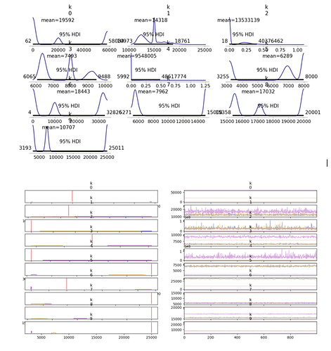
If you let me know which stats would be most helpful, I can provide those. Here’s a selection below. The max tree depth was something I was playing with. In the image below it tends to upper values but I have ran models where it remains below 9.

[jessegrabowski]

This simple example samples with NUTS on my machine:

with pm.Model() as m:
    x1 = pm.Normal('x1', size=(2, 2))
    x2 = pm.Normal('x2', size=(2, 2))
    mu = pt.linalg.block_diag(x1, x2)
    
    obs = pm.Normal('obs', mu=mu, sigma=1, observed=np.random.normal(size=(100, 4, 4)))
    idata = pm.sample()

Can you share exactly what you are running? I also don’t see a call to pm.linalg.solve in your code, but the error you are getting relates to that. Your results for eta are extremely precise, which is really strange. I am wondering if your matrix is being sample as low-rank, and this is causing the problems. You could try adding a small jitter (like 1e-8) to the diagonal of whatever you’re inverting to keep it PSD and avoid these numerical problems?

[mmn]

Same here - the sample code you gave works no problem.

Also I omitted the line where I used pm.linalg.solve. I have edited that now in the main post.

I can provide the full code but it’s best I chop it down a bit as there’s a fair few lines to it in forming the observation.

[mmn]

Hi @jessegrabowski and others

A few updates on this (though problems persist).

1. I realised my block diagonals need to be created within a scan file to preserve gradients. In numpy-speak, my arrays are 3D - they are 2D arrays but have a frequency dependency (hence a need for 3D). I therefore needed to construct the block-diag accordingly. A silly mistake really.

2. Selecting different samplers yields some changes, numpyro produced nice-looking distributions…

Nutpie less so…

SMC didn’t look too pretty either…

3. From a sampling time perspective, the above methods still range within the 4-7 hour mark. I have investigated the bottleneck by limiting the likelihood/observation relationships to different points of my calculation, and seeing how long it takes to compute the MAP. As soon as anything involving an inversion, or something which computes it via alternatives is used, I get a slow down.

4. On the inversion, I’ve been looking at some alternatives:

• pt.linalg.solve seems to work well, is quicker than pt.linalg.inv, but improvements on the 4-hour mark do not appear.
• I have tried SVD and QR decomposition also, but sampling seems to default once more to Powell. It may be that I am doing something wrong but it is not immediately obvious.

Below is a sample code, I’ve added some downloadable arrays in the hope of keeping it as concise as possible.

Please note I have included sections of commented-out code to illustrate the different effects of each method to a) construct the block diagonal and b) compute the inverse of a bracketed term - suspected to be root of the slowdown

data.npy (689.2 KB)
Yfull_with_zeros.npy (689.2 KB)
Y1.npy (189.2 KB)
Bt_inv.npy (328.3 KB)
B_inv.npy (328.3 KB)
Bt_shared.npy (328.3 KB)
B_shared.npy (328.3 KB)

I hope that the above and code below is clear,. I am happy to provide more information if needed.

Thank you!

import numpy as np
import pymc as pm
import pstats
import cProfile
import io
from pytensor import shared
from scipy import stats
import numpy.matlib
from pytensor.tensor.linalg import block_diag as block_diag_pt
import pytensor.tensor.slinalg
import pytensor.tensor.nlinalg
from scipy.linalg import block_diag
from pymc import pytensorf
import pytensor
import pytensor.tensor as pt
from pytensor import function
import matplotlib.pyplot as plt
import arviz as az
import timeit
import time

az.style.use("arviz-plasmish")
plt.close('all')

pytensor.config.exception_verbosity = 'high'

""" define and load data """
f = np.logspace(np.log10(10), np.log10(100), 50)  # Frequency array
w = 2*np.pi*f 

load_observation_data = np.load('data.npy')
load_Y1 = np.load('Y1.npy')
load_Y1_zeros = np.load('Yfull_with_zeros.npy')
load_B = np.load('B_shared.npy')
load_Bt = np.load('Bt_shared.npy')
load_Bt_inv = np.load('Bt_inv.npy')
load_B_inv = np.load('B_inv.npy')
 
num_coupled = 10
num_uncoupled = 21


""" true values to be inferred """
k_true = [20000, 15000, 10000, 8000, 6000, 8000, 10000, 15000, 20000, 25000]
eta_true = [0.2, 0.1, 0.1, 0.08, 0.06, 0.08, 0.09, 0.15, 0.2, 0.25]

input_combined = k_true + eta_true
input_dims = int(len(input_combined) / 2)


""" Sharing and preparing variables for pymc (tensor reassignement / vectorising etc) """
winv_pt = pt.as_tensor_variable(1/w)  # , kwargs)
Y_mat_shared = pt.as_tensor_variable(load_Y1)
data = pt.as_tensor_variable(load_observation_data.flatten())
B_pymc = pt.as_tensor_variable(load_B)
Bt_pymc = pt.as_tensor_variable(load_Bt)
B_inv_pymc = pt.as_tensor_variable(load_B_inv)
Bt_inv_pymc = pt.as_tensor_variable(load_Bt_inv)

""" zero matrices outside pm,model """
# # Empty list 
Z_pt = []
Y_pt = []
Y_isol_pt = []
Y_isol_pt_alt = []
det_Z_pt = []
Y_i_matrix_pt = pt.zeros((len(f), 2*num_coupled, 2*num_coupled))
Y_fill_limit = 2*num_uncoupled - 2*num_coupled
Y_full_zeros = pt.zeros((len(f), 2*num_uncoupled, 2*num_uncoupled))
Y_full = pt.set_subtensor(Y_full_zeros[:,0:Y_fill_limit, 0:Y_fill_limit], Y_mat_shared)

#%%
t1 = time.time()

with pm.Model() as model:
    # Priors for unknown model parameters
    k = pm.LogNormal("k", mu=np.log(10000), sigma=1, shape=(10,))
    eta = pm.Beta("eta", alpha=2, beta=2, shape=(10,))
    sigma = pm.HalfNormal("sigma", 0.1)
       
    det_Z = 1 / ((k * winv_pt[:, None])**2 * (1 + eta**2))
    Y11 = (k * eta * winv_pt[:, None]) * det_Z
    Y12 = (-k * winv_pt[:, None]) * det_Z
    Y21 = (k * winv_pt[:, None]) * det_Z
    Y22 = (k * eta * winv_pt[:, None]) * det_Z

    # Construct 2 x 2 matrices
    upper_stack = pt.stack([Y11, Y12], axis=2)  # shape (len(w), num_coupled, 2)
    lower_stack = pt.stack([Y21, Y22], axis=2)  # shape (len(w), num_coupled, 2)
 
    # Fill each 2x2 block into the correct diagonal position (create block diagonal)
   
    for i in range(num_coupled):  # num_coupled should be 10 here
        idx = 2 * i
        Y_i_matrix_pt = pt.set_subtensor(
            Y_i_matrix_pt[:, idx:idx+2, idx:idx+2],
            pt.stack([
                pt.stack([Y11[:, i], Y12[:, i]], axis=1),
                pt.stack([Y21[:, i], Y22[:, i]], axis=1)
            ], axis=1)
        )
    """ Assemble Y_full - 2 Options considered """
    # Option 1 to assemble Y_full - pre allocate a matrix/tensor with zeros and use set_subtensor to fill in entries.
    # index = Y_mat_shared.eval().shape[1]
    # Y_full = pt.set_subtensor(Y_full[:, index:index+2*num_coupled, index:index+2*num_coupled], Y_i_matrix_pt)
    
    # Option 2 to assemble Y_full - use block diagonal (has to be within a scan function otherwise no NUTS)
    def step(Y_mat_shared, Y_i_matrix_pt):
        return  block_diag_pt(Y_mat_shared,Y_i_matrix_pt)
   
    Y_full, _ = pytensor.scan(fn=step, sequences=[Y_mat_shared, Y_i_matrix_pt], outputs_info=None)#, non_sequences=[B_pymc, ,])

    """ Determine the inverse of the bracketed element - 4 Options considered """   
     
    # Option 1 to compute bracket inverse without scan - Perform a vectorised calculation, 
    # relying on 'pt.linalg.solve' to avoid direct use of matrix inverse
    bracket_pt = B_pymc @ Y_full @ Bt_pymc
    inverse_bracket = pt.linalg.solve(bracket_pt, pt.eye(bracket_pt.shape[1]))
 
    # Option 2 - Use a QR decomposition - DEFAULTS TO POWELL
    # def step_QR(B_pymc, Y_full, Bt_pymc):
    #     bracket_pt = B_pymc @ Y_full @ Bt_pymc
    #     Q,R = pt.linalg.qr(bracket_pt,mode="complete")
    #     # Compute the inverse of R
    #     # R_inv = pt.linalg.inv(R)
    #     R_inv = pt.linalg.solve(R, pt.eye(R.shape[1]))
    #     # Compute the inverse of A using Q and R
    #     bracket_pt_inverse = R_inv @ Q.T  # Since Q is orthogonal, Q^-1 = Q^T
    #     return  bracket_pt_inverse #pt.linalg.solve(bracket_pt, pt.eye(bracket_pt.shape[1]))# Y_full - Y_full @ Bt_shared @ inverse_bracket @ B_pymc @ Y_full

    # inverse_bracket,_  = pytensor.scan(fn=step_QR, sequences=[B_pymc, Y_full, Bt_pymc], outputs_info=None)#, non_sequences=[B_pymc, ,])
    
    # Option 3 - Use a SVD decomposition - DEFAULTS TO POWELL
    # def step_SVD(B_pymc, Y_full, Bt_pymc):
    #     bracket_pt = B_pymc @ Y_full @ Bt_pymc
    #     svd_result = pt.nlinalg.svd(bracket_pt)
    #     u, s, v = svd_result
    #     bracket_pt_inverse = pt.nlinalg.matrix_dot(v.T, pt.nlinalg.matrix_dot(pt.diag(s**-1), u.T))
  
    #     return bracket_pt_inverse  # The inverse of bracket_pt
    
    # inverse_bracket, _ = pytensor.scan(fn=step_SVD, sequences=[B_pymc, Y_full, Bt_pymc], outputs_info=None)
   
    # Option 4  - do everything in scan 
    # relying on 'pt.linalg.solve' to avoid use of matrix inverse
    # def step_Yc(B_pymc, Y_full, Bt_pymc):
    #       bracket_pt = B_pymc @ Y_full @ Bt_pymc
    #       inverse_bracket = pt.linalg.solve(bracket_pt, pt.eye(bracket_pt.shape[1]))
    #       Yc_pt = Y_full - Y_full @ Bt_pymc @ inverse_bracket @ B_pymc @ Y_full
    #       return Yc_pt  # The inverse of bracket_pt
     
    # Yc_pt, _ = pytensor.scan(fn=step_Yc, sequences=[B_pymc, Y_full, Bt_pymc], outputs_info=None)
    
    """ compute Yc_pt / likelihood """
    Yc_pt = Y_full - Y_full @ Bt_pymc @ inverse_bracket @ B_pymc @ Y_full
    likelihood = pm.Normal("likelihood", mu=pt.flatten(Yc_pt), sigma=sigma, observed=data)#pt.as_tensor_variable(inv_bracket_check_c2r.flatten()))
     
    """ Find MAP if necessary - this is not required for NUTS but useful to speed check """

    t2 = time.time()
    map_estimate = pm.find_MAP()
    print(map_estimate['k'])
    print(map_estimate['eta'])
    elapsed2 = time.time() - t2
    print('elapsed2', elapsed2)
        
    """ Sampling with SMC """
    # trace_smc = pm.sample_smc(draws=2000, chains=16, cores =16, progressbar=True, parallel=True, random_seed=42)
   
    """ NUTS-based sampling (I have tried pymc, nutpie, numpyro"""
#     trace = pm.sample(
#         1000, 
#         tune=1000, 
#         chains=4, 
#         cores=15,
#         # nuts={"max_treedepth": 15},
#         nuts_sampler='numpyro',
#         return_inferencedata=True,
#         discard_tuned_samples=False,
#         random_seed=42
#     )


# elapsed1 = time.time() - t1
# print('elapsed1', elapsed1)

[aseyboldt]

Hello,

thanks for the full code, always nice to have something I can run
I’m not sure what the context is, but I noticed things in the code that look to me like they could possibly be bugs. Before I look closer, could you check if that’s so? Would be a shame to look into it further only to find out that there was a typo in the code.

A draw from the assembled matrix Y_full looks like this if I run it on my machine:

generated using

import seaborn as sns
sns.heatmap(Y_full.eval()[0], center=0)

Is that correct, or did you want to have the 2x2 blocks along the diagonal?

This here looks a lot like the woodbury identity to me (especially because I think Y_full is supposed to be an inverse of some kind?), but if so, aren’t you missing an identity matrix in the bracket?

Yc_pt = Y_full - Y_full @ Bt_pymc @ inverse_bracket @ B_pymc @ Y_full
# should this be this?
Yc_pt = Y_full - Y_full @ Bt_pymc @ inv(identity + B Y_full Bt) @ B_pymc @ Y_full

[mmn]

Hey @aseyboldt - thanks for the reply. I like the heatmap trick too

Which method did you use to construct Y_full? In the code, there are 2 methods.

Method 1 takes a variable Y_mat_shared and places it in the top left of an otherwise zero matrix (again - numpy speak). The code within the model context fills the diagonals from row/column 22 onwards with 2 x 2 matrices.

Before the model context, Y_full looks like this (partially) - similar to what you presented in the screen grab.

but within the model it fills the diagonals from row/col 22 onwards with Y_i_matrix_pt. It should (correctly I hope) look like this…

Method 2 takes the Y_mat_shared and Y_i_matrix_pt elements and constructs a block diagonal matrix using the block_diag command without preallocating and then filling the empty array. I learned that I need to do this within a scan to keep gradients in play.

As for the expression, it does indeed look like the Woodbury identity (which I did consider as part of reducing the inverse operation load) but it is an expression for structural coupling.

Happy to field any more questions - or go bug hunting!