Puzzled about the array ordering of LKJCC corr as xarray object

[jonsedar]

I might be losing my mind here, would definitely appreciate input from a kind soul.

I think I’ve misunderstood xarray indexing, but there could be something else going on too. This question has become apparent during my plotting model posteriors.

Background

I have a model that uses an LKJCholeskyCov to create an MvNormal. I name the dims, and I use the unpacked compute_corr=True parameter to leave me a useful _corr in the trace.

Relevant code fragment:

self.coords.update({'b0_names': ['gc_omega_b0', 'gc_theta_b0', 'ulr_b0']})
...
sd_dist = pm.InverseGamma.dist(alpha=11, beta=10) 
chol, corr_, stds_ = pm.LKJCholeskyCov('lkjcc', n=3, eta=2, 
                                       sd_dist=sd_dist, compute_corr=True)
b0 = pm.MvNormal('b0', mu=0, chol=chol, dims='b0_names')

After sampling I can plot posteriors for b0:

axs_pp = az.plot_pair(mdlb6.idata, var_names=rvs, divergences=True, 
                                   marginals=True, figsize=(5, 5))

Observe:

• There appears to be positive correlation between ulr_b0 and gc_theta_b0 (the others are negative), and in conventional lower triangle array indexing, this is plotted at index 4:

[[0 - -]
 [1 2 -]
 [3 4 5]]

• If I want the 2D i, j index for this I can use np.tril_indices and b0_names and recreate the axis labels shown on the plot. Just to confirm, index 4 is where i=2, j=1, and the relevant pair of b0_names is ('ulr_b0', 'gc_theta_b0'), and the plot shows xlabel='b0\ngc_theta_b0'

i, j = np.tril_indices(n=3, k=-1)
print(i, j)
> [1 2 2] [0 1 1]

[(coords['b0_names'][a], coords['b0_names'][b]) for a, b in zip(i, j)]
> [('gc_theta_b0', 'gc_omega_b0'),
> ('ulr_b0', 'gc_omega_b0'),
> ('ulr_b0', 'gc_theta_b0')]

axs_pp[2][1]
> <AxesSubplot:xlabel='b0\ngc_theta_b0'>

• Finally to note if I read along i, j I can say the order of paired correlations is [negative, negative, positive]

• All good so far

My surprise observation

If I now use i, j to index lkj_corr and then plot_posterior, I get plots that appear to show a reversed order [positive, negative, negative]:

axs = az.plot_posterior(
        mdlb6.idata.posterior['lkjcc_corr'].values[:, :, i, j], 
        ref_val=[0, 0, 0], figsize=(12, 2))

… I can plot this in my expected order if I reverse i and j and then index lkjcc_corr

axs = az.plot_posterior(
        mdlb6.idata.posterior['lkjcc_corr'].values[:, :, i[::-1], j[::-1]], 
        ref_val=[0, 0, 0], figsize=(12, 2))

Just to isolate this further, let’s view index 4 as above where i=2, j=1… yep that’s definitely not what I expected

axs = az.plot_posterior(
        mdlb6.idata.posterior['lkjcc_corr'].values[:, :, 2, 1], 
        ref_val=[0, 0, 0], figsize=(8, 2))

If I view the xarray in Notebook, the dimensions look reasonable to me and the lowest 2D unit of dimensions is 3x3, has an identity diagonal - it looks as I would expect. Obviously this means that merely swapping i, j would get the same mirrored value from the upper triangle, so the order doesn’t matter

Even more concretely

It seems that when I try to index so as to get cell 4, I instead get cell 1, which is a “flip and rotate” or a mirror around the anti-diagonal

e.g.

a = np.array([
    [0, np.nan, np.nan],
    [1, 2, np.nan],
    [3, 4, 5],
    ])
print(a)
i, j = np.tril_indices(n=3, k=-1)
print(i, j)
print(a[i[-1:], j[-1:]])

print(b)
b = np.rot90(np.fliplr(a), k=3)
print(b[i[-1:], j[-1:]])

>>
[[ 0. nan nan]
 [ 1.  2. nan]
 [ 3.  4.  5.]]
[1 2 2] [0 0 1]
[4.]
[[ 5. nan nan]
 [ 4.  2. nan]
 [ 3.  1.  0.]]
[1.]

My stupid question

Does lkjcc_corr somehow have an inverted index?

Or: what have I misunderstood about xarray indexing?

Many thanks if you made it this far!

Relevant env details:

pymc3=3.11.4
arviz=0.12.1

[OriolAbril]

@jonsedar

It seems that when I try to index so as to get cell 4, I instead get cell 1, which is a “flip and rotate” or a mirror around the anti-diagonal

The anti-diagonal symmetry makes me suspect this is an issue with order="F" or order="C" when unpacking the cholesky or something of the sort. It is indeed very odd.

The missmatch is between the results shown in plot_pair and in the correlations stored in corr, however, due to xarray being involved and the mixture of positional and label based indexing the situation is a bit more puzzling.

I’d recommend you use idata_kwargs to also define the dims in corr. That should look like:

b0_names = ['gc_omega_b0', 'gc_theta_b0', 'ulr_b0']
self.coords.update({'b0_names': b0_names, "b0_names2": b0_names})
...
    idata_kwargs={"dims": {"lkjcc_corr": ["b0_names", "b0_names2"]}},

something very similar is done in the model at https://www.pymc.io/projects/examples/en/latest/case_studies/multilevel_modeling.html that uses LKJ too.

That will have the corr variable have meaningful labels instead of the default assigned dimensions. I would then do two things:

corr_means = idata.posterior["lkjcc_corr"].mean(("chain", "draw"))
corr_means.sel(b0_names="gc_omega_b0", b0_names2="ulr_b0")

does this match the correlation for that plot in plot_pair?

Another thing you can try is instead of looping using the tril_indices to call plot_posterior you can try the approach from Label guide — ArviZ dev documentation, do the labels here and in plot_pair match?

[jonsedar]

Thanks Oriol, I’d hoped you might have a few good suggestions!

I’ll try those tomorrow and report back…

[jonsedar]

Hmmm interesting, I think there’s some indexing weirdness somewhere, and have an ill-educated suggestion at the end…

My path so far:

(with mild brainache from trying to get my head around xarray, ha)

(1) I fed my model object (and then az.from_pymc3 aka az.data.io_pymc3_3x.from_pymc3 in my v3 usage) with the dims as you suggested:

# snippets involved
...
b0_names = ['gc_omega_b0', 'gc_theta_b0', 'ulr_b0']
...
idata_kwargs = {'dims': {'lkjcc_corr': ['b0_names', 'b0_names2']}}
...
coords.update({'b0_names': b0_names, 'b0_names2': b0_names})
...
k.update(**idata_kwargs)
az.from_pymc3(**k)

… the model samples fine and the posterior idata looks as intended: with coords b0_names and b0_names2 in the right order.

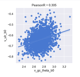
(2) The pairs plot looks the same as I inserted above, so I also wanted to make sure my eyes aren’t playing tricks on me and the position 4 subplot really is positive:

v_ulr_b0 = mdlb6p.idata.posterior['b0'].sel(b0_names='ulr_b0').stack(dims=('chain', 'draw')).values
v_gc_theta_b0 = mdlb6p.idata.posterior['b0'].sel(b0_names='gc_theta_b0').stack(dims=('chain', 'draw')).values
from scipy import stats
rho, _ = stats.pearsonr(v_gc_theta_b0, v_ulr_b0)
f, axs = plt.subplots(1, 1, figsize=(4, 4))
ax = sns.regplot(x=v_gc_theta_b0, y=v_ulr_b0, ax=axs)
_ = ax.set(title=f'PearsonR = {rho:.3f}', xlabel='v_gc_theta_b0', ylabel='v_ulr_b0')

… yep thats the same plot, so the b0 selection is named correctly (and now we have an approximate correlation value to look for +0.3)

In fact here’s all 3 for reference:

(3) I now select from lkjcc_corr as you suggested, remembering that the order doesn’t matter (we could equally do b0_names='gc_theta_b0', b0_names2='ulr_b0')

corr_means = mdlb6p.idata.posterior["lkjcc_corr"].mean(("chain", "draw"))
corr_means.sel(b0_names='ulr_b0', b0_names2='gc_theta_b0')

… we get -0.18, that’s definitely not a positive correlation value

(4) A quick triple check using alternative indexing:

mdlb6p.idata.posterior['lkjcc_corr'].values[:, :, 2, 1].mean()
> -0.18642255020919818

mdlb6p.idata.posterior['lkjcc_corr'].loc[:, :, 'ulr_b0', 'gc_theta_b0'].mean()
> <xarray.DataArray 'lkjcc_corr' ()>
array(-0.18642255)
Coordinates:
    b0_names   <U11 'ulr_b0'
    b0_names2  <U11 'gc_theta_b0'

(5) Okay what about the others? Where’s the positive value around 0.3 ?

There it is, in lower-triangle position 1, aka i=1, j=0 aka

corr_means.sel(b0_names='gc_omega_b0', b0_names2='gc_theta_b0')

> array(0.31553846)

…

So, I think I’ve ruled out indexing issues and coords and dims. The lkjcc_corr matrix appears to be flip-rotated, or the indexing has been reversed along each axis somehow

---

At this point I start to run out of ideas…

I’ve looked into the code that generates the corr (permalink to v3 branch that I’m using) (note that the v4 code uses the same logic)

        chol = pm.expand_packed_triangular(n, packed_chol, lower=True)
        # compute covariance matrix
        cov = tt.dot(chol, chol.T)
        # extract standard deviations and rho
        stds = tt.sqrt(tt.diag(cov))
        inv_stds = 1 / stds
        corr = inv_stds[None, :] * cov * inv_stds[:, None]
        if store_in_trace:
            stds = pm.Deterministic(f"{name}_stds", stds)
            corr = pm.Deterministic(f"{name}_corr", corr)

Is is possible that the tt.dot does a flip-rotate? Or perhaps the indexing for inv_stds is in the wrong order and we want something like corr = inv_stds[:, None] * cov * inv_stds[None, :] ?

I’ll try a couple of things this end…

---

<EDIT #1 additional exploration>

Right, so I can easily replicate the calculations for lkjcc_corr outside of the model by just reusing that code as:

packed = mdlb6p.idata.posterior['lkjcc'].mean(('chain', 'draw')).values
print(packed)  # so you can replicate

> [ 0.98541743  0.43684498  1.25796973 -0.10103472 -0.14227276  0.75882839]

n = 3
out = np.zeros((n, n))
idxs = np.tril_indices(n)
# hacky version of tt.set_subtensor
for p, tup in enumerate(zip(*idxs)):
    out[tup] = packed[p]

chol = out.copy()
cov = np.dot(chol, chol.T)
stds = np.sqrt(np.diag(cov))
inv_stds = 1 / stds
corr = inv_stds[None, :] * cov * inv_stds[:, None]
print(corr)

> [[ 1.          0.32804515 -0.12975902]
   [ 0.32804515  1.         -0.2151765 ]
   [-0.12975902 -0.2151765   1.        ]]

Which looks broadly the same to me. I’m at a loss…

---

<EDIT #2 mucking around with flip-rotate on cov and pretty much out of my depth, and trying to relearn matrix math…>

In the above code snippet, if I flip rotate cov, I do get the ordering I would expect:

cov = np.rot90(np.fliplr(cov), k=3)
...
print(corr)

> [[ 1.         -0.2151765  -0.12975902]
   [-0.2151765   1.          0.32804515]
   [-0.12975902  0.32804515  1.        ]]

Is this interesting? maybe…

The code uses tt.dot(), but since these are 2D matrices, it would be more appropriate (following the numpy concept) to use tt.matmul which doesn’t exist

If it did exist, I might try to play with the order kwarg, which does exist in numpy, so let’s play with it in numpy:

cov = np.matmul(chol, chol.T, order='K')
cov1 = np.matmul(chol, chol.T, order='C')
cov2 = np.matmul(chol, chol.T, order='F')

print(cov == cov1)
print(cov == cov2)

> [[ True  True  True]
   [ True  True  True]
   [ True  True  True]]
  
  [[ True  True  True]
   [ True  True  True]
   [ True  True  True]]

… nope that’s not it, and I’m starting to lose the plot!

[OriolAbril]

can you share the whole model? Or a minimal example that uses LKJCholeskyCov in a similar way?

I am now realizing that in the pieces of code you shared, b0 is not observed, so its posterior samples won’t generally match draws of the distribution we have defined as prior. The prior mean of b0 is 0 for all components yet no posterior sample is close to 0 for any of them and that is exactly what we want!

lkjcc is a hyperprior which always makes things harder to wrap one’s head around, but a prior nonetheless; if you had used a hardcoded prior you would not be trying to match the correlations of the b0 posterior samples to the correlations defined by the prior (our you would be but only to see if they were exceedingly different which could point at prior/data incompatibilities).

Also, sorry for the previous sending on wild-goose chase message with dims and indexing.

[jonsedar]

Hey Oriol, thanks for coming back to it - much appreciated!

I don’t think that was a wild goose chase though - I still don’t understand why the PearsonR on b0 is flip-rotated from the correlations in lkjcc_corr…

In any case, a simplified, pooled version looks a bit like the following… I hope this helps (and I hope moreover that it’s not fatally flawed since it comes from a couple of papers and seems to work for me so far! Haha).

This is a parametric approximation of a claims development curve where the cumulative sum lr_csum_ci of claims increases (generally speaking) over time t for a cohort of insurance policies.

We observe only the value of lr_csum_ci (here as a Lognormal), but decompose the median into two components:

1. A development curve here implemented as a Fisk (log-logistic) CDF that transforms t: _fisk_cdf(gc_omega, gc_theta, t), ranges [0, 1] has support on t in (0, +inf)
2. An expected loss ratio (ELR), has support on (0, +inf)

This is a useful decomposition for parameter interpretation / decision-making / setting priors according to business plan etc

So b0 is not directly observed - actually maybe I ought to non-center that, per the docs. Also note I don’t actually use corr_ (lkjcc_corr) for anything.

# handle data
y = pm.Data('y', obs['lr_csum_ci'].values, dims='obs_id')
t = pm.Data('t', obs['duration'].values + 1, dims='obs_id')

# correlated hyperpriors for GC and ELR intercept
sd_dist = pm.InverseGamma.dist(alpha=11, beta=10, shape=3)
chol, corr_, stds_ = pm.LKJCholeskyCov('lkjcc', n=3, eta=2, 
                              sd_dist=sd_dist, compute_corr=True)
b0 = pm.MvNormal('b0', mu=0, chol=chol, dims='b0_names')

# growth curve (cumulative) log-logistic (Fisk) CDF
gc_omega = tt.exp(b0[0])  # omega (slope at median)
gc_theta = tt.exp(b0[1])  # theta (median)
# elr
elr = tt.exp(b0[2])

yhat_s = pm.InverseGamma('yhat_s', alpha=101, beta=10)
yhat_s_w = yhat_s / (1 + (t / 40))  # weighting toward later developments
_ = pm.Lognormal(
    'yhat',
    mu=tt.log(_fisk_cdf(gc_omega, gc_theta, t) * elr),
    sigma=yhat_s_w,
    observed=y,
    dims='obs_id',
)

Cheers!

[OriolAbril]

Why do you expect the correlation of b0 to be lkjcc_corr?

Here you have one “group” only, but as I said, lkjcc is a hyperprior and the MvNormal with covariance lkjcc is a prior.

If instead of using MvNormal as the prior for b0 you used a Normal one, would you expect them to be uncorrelated?

If instead of using lkjcc as covariance of the MvNormal you used a fixed value, would you expect the correlation of the posterior samples in b0 to be that fixed value?

If instead of having a single “group” you used the lkjcc with a hierarchical model, would you expect the correlations of all levels to match lkjcc? This is actually what happens in A Primer on Bayesian Methods for Multilevel Modeling — PyMC example gallery, the correlations in posterior samples between a and b in ab_county for each county go between -0.6 and -0.1.

Your case is similar to the model in the radon notebook that uses lkjcholeskycov, but you only have one “group” in your case. I generally struggle trying to interpret and intuitively work with hyperpriors, but I don’t see why does lkjcc_corr need to match the correlations between posterior samples. It might seem that the fact there is only one group means the hyperprior will learn the correlations in b0, but:

• does it really have enough information to do so? Has it really learned the correlations but it stores them in the wrong position? [1]
• Does it get stuck on some kind of local minima? After all, lkjcc is “just a prior”, the vast majority of models only use univariate priors yet the vast majority of posteriors have correlations between the posterior variables.
• Does the model show any sign of not having converged? There are many cases when we can know it hasn’t converged but never really get any convergence guarantee.

[1]. Instead of comparing the pdfs of each of the non-diagonal positions in lkjcc_corr to the mean correlation between variables in b0, you can use subsampling bootstrap (if you have 1000 samples, take the first 100 and compute the correlation, then the 1-101, 2-102… so you get 900 values of the posterior correlation) to estimate the pdf of the correlations in b0 and see if the distributions do indeed look the same but in the wrong matrix position or if they don’t.

[jonsedar]

Hi Oriol, thanks for the detailed reply!

You raise lots of good points, and I’m not disagreeing with you - I’ve no reason to suspect the matrix indexing is wrong per se. Will try out the subsampling bootstrap and report back.

I think I’ll have to create a synthetic dataset biased in ways I know precisely - and see what happens to that.

As to your conceptual questions, this could be my misunderstanding, but I’m slightly uneasy to see that the posterior lkjcc_corr seems to disagree (in sign) with the empirical correlation of the posteriors on b0.

Hopefully to draw analogy: in the simplest case of:

m1 = pm.Normal('m1', mu=0, sigma=1)
m2 = pm.Normal('m2', mu=m1, sigma=1, shape=3)

… I would expect the posterior mean of hyperparam m1 to represent the weighted mean of the posterior 3 levels in m2

I think this is analogous to:

chol, corr_, stds_ = pm.LKJCholeskyCov('lkjcc', n=3, eta=2.0, 
                          sd_dist=sd_dist, compute_corr=True)
b0 = pm.MvNormal('b0', mu=0, chol=chol, dims='b0_names')

… since even though we’re not hierarchical on the mu of b0, the posterior lkjcc_corr is (indirectly via chol) fed into b0. If lkjcc_corr is not fixed to e.g. 0, but is free to move, is it really plausible that the lowest energy state for those posteriors would be a different sign to those of the MvN posteriors that they directly feed?

Perhaps a quick test will be to feed lkjcc_corr into b0. I’ll try that later on today