State Space Models in PyMC

I am working with a time series data (regional employment) that has many missing values, but that also has a hierarchical structure, such that observed data points contain information about the missing data. Rather than just use a SARIMAX with kalman filter setup, I am curious to know if I can solve the problem in PyMC.

In that spirit, I wrote down a local level model to test my intuition about how a state space model would look in PyMC. I am trying to adhere to the general matrix form of the SSM as closely as possible, because I am hoping to get to a general framework I can use for much more complicated problems.

coords = {'time':nile.index.year.values,
          'states':['level', 'trend']}

def step_statespace(epsilon, x, A):
    x_ = tt.dot(A, x) + epsilon
    return x_

with pm.Model(coords=coords) as nile_model:
    sigma_level = pm.HalfNormal('sigma_level', sigma=1)
    sigma_trend = pm.HalfNormal('sigma_trend', sigma=0.05)
    x0 = pm.Normal('x0', mu=np.zeros(2), sd=np.ones(2), dims=['states'])
    
    epsilons = pm.Normal('epsilons', 
                           mu=np.zeros(2), 
                           sigma=tt.stack([sigma_level, sigma_trend]),
                           dims=['time', 'states'])
    
    A = tt.as_tensor_variable(np.array([[1.0, 1.0], 
                                        [0.0, 1.0]], dtype='float32'))
    
    F = tt.as_tensor_variable(np.array([[1.0 ,0.0]], dtype='float32'))
    
    state_history, _ = theano.scan(fn=step_statespace,
                                   sequences=epsilons,
                                   outputs_info=x0, 
                                   non_sequences=A)
    
    hidden_states = pm.Deterministic('hidden_states', state_history, dims=['time', 'states'])
    observed_states = pm.Deterministic('observed_states', (hidden_states * F).sum(axis=-1), dims=['time'])
    
    sigma_observed = pm.HalfNormal('sigma_height', sigma=1.0)
    
    height = pm.Normal('height', 
                      mu=observed_states,
                      sigma=sigma_observed,
                      observed=nile.values.ravel(),
                      dims=['time'])
    
    nile_prior = pm.sample_prior_predictive(var_names=['height', 'hidden_states'])

This model samples very poorly. It takes at least 20 minutes and diverges like crazy. Prior checks look OK, and shapes check out. When I run the scan in pure theano things work fine, so I think it’s a problem with how I’m setting up the random variables? The code is quite similar to “Local level - Nile” State Space Model (Kalman Filter) in PyMC3, and in the linked notebook there the model samples quite quickly (but still has many divergences, that seems to be a requirement for PyMC example notebooks…). One major difference is that I’m doing a dot-product in the step_statespace function, and keeping track of the hidden state.

(As an aside, computing the observed state as a dot product, tt.dot(F, hidden_states) causes the “cannot pickle a fortran object” error on Windows. I thought that was quite odd!)

One question I have is whether the shape of epsilons, the innovation series, should be T x k or just 1 x k. When I test the scan function in pure Theano i need T innovations of course, but it’s not clear to me how the internals of the random variable works. Suppose I pass a 1xk random variable as a non_sequence to scan. During a single iteration of sampling, is the random variable sampled once, then the whole scan run, or is the random variable re-sampled at every scan step?

One question I have is whether the shape of epsilons, the innovation series, should be T x k or just 1 x k.

The standard way would be to make the innovations be independent for each time point, so T x k.

During a single iteration of sampling, is the random variable sampled once, then the whole scan run, or is the random variable re-sampled at every scan step?

With a non_sequence argument to scan, it won’t be resampling at every timestep - it’s just sampled once.

2 Likes

That’s what I figured, thanks.

I’ve been thinking about this and playing with it as time permits, and I wonder if there is a work-around to save the sampler a lot of hassle. The innovations aren’t just independent between timesteps – for all traditional statistical time series models that can be cast into a state-space format (SARIMAX, VARMAX), the distribution over innovations is assumed to be stationary. Any non-stationary dynamics (MA components, for example) can be modeled in the state or observation equations to render the noise stationary.

Perhaps I have a fundamental misunderstanding about what happens when a random variable is given a shape. When I implement a T x k innovation series, I am forcing the sampler to estimate a huge number of nuisance parameters, when in fact I only need to know the parameters that describe the transition and observation noise. It’s also not obvious to me what these epsilons are in the statespace framework.They aren’t quite residuals, because those are associated with the observation noise. They seem to me just an artifact of how I’m implementing the model.

What that in mind, I wonder if there is a better way to write it? Really the hidden states should be the random variables with mean defined autoregressively and constant variance.

I feel your pain. For systems with discrete hidden state, there are now very fancy tools for summing those states out to eliminate all the nuisance parameters.

It’s also not obvious to me what these epsilons are in the statespace framework.

Economists, roboticists, and ecologists will probably all use different terms and interpretations for those values in their respective subfield usages of SSMs. Much of the time series literature elides those random variables because the estimation equations can be written without them explicitly.

Unfortunately, there’s probably not a silver bullet within the MCMC world for getting what you want, as dealing with these nuisance variables requires integrating out all T x k variables… If you want something that is very fast, you can use the forward-backward smoother as part of a larger MCMC scheme. That’s what I’ve done in this repository. That way, you sample all of the internal states extremely quickly using a closed-form solution, and use NUTS for everything else.

1 Like

Exactly so, and I guess I should have been more precise with my language. Certainly some more elaborate models (in economics at least, where I have an iota of a clue) put interpretable meaning to the random shocks. It’s just unusual to talk about the unobserved technology shock to production in 1992, since the usual object that is discussed is the distribution of these shocks over the whole time series. But, now that you mention it, people do do shock decomposition, so I guess we get that decomposition “for free” by estimating T x k epsilons.

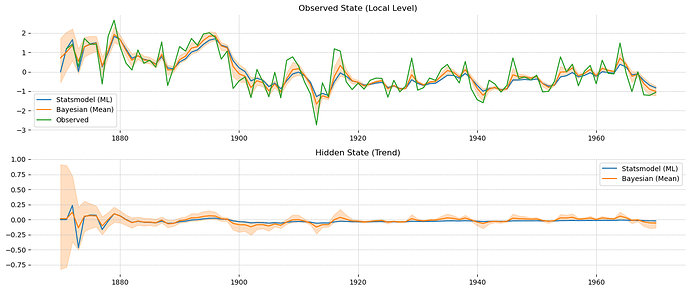
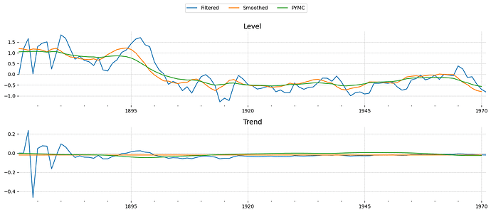
One thing I didn’t understand first looking at the output graphs was that the PyMC state estimates are much closer to the smoothed Kalman states than to the filtered ones. In principal, this should not be the case, since there’s no integration of future information into the PyMC model. Is this resemblance just superficial, caused by the fact that the innovation series is embedded in the filtered results?

Also, thank you for linking your repository, it looks extremely relevant to the types of problems I’m working on. I’ll have a look at what you’ve done and try to learn from it, or give up and try to use it directly!

One thing I didn’t understand first looking at the output graphs was that the PyMC state estimates are much closer to the smoothed Kalman states than to the filtered ones. In principal, this should not be the case, since there’s no integration of future information into the PyMC model.

The way you’ve written the generative AKA forward model is one-step-at-a-time from past to present, but the inference in PyMC is indeed making use of all future knowledge to infer the innovations / shocks at any single point in time.

1 Like

Interesting. Is this unavoidable? Should I care?

I thought a different angle might be to just implement a Kalman filter in Aesara and use it with pm.Potential to get the model’s likelihood.

I am definitely missing something when it comes to defining an Op, because the shapes are not working out at all. Here’s what I have for the filter:

class KalmanLikelihood(at.Op):

    itypes = [at.dmatrix, 
              at.dmatrix,
              at.dmatrix,
              at.dmatrix,
              at.dmatrix,
              at.dmatrix,
              at.dmatrix]
    
    otypes = [at.dmatrix, at.dmatrix, at.dscalar]

    def __init__(self, data):
        self.data = data
        self.kalman_filter = self._build_kalman_filter()
                        
    def _build_kalman_filter(self):
        """
        Construct the computation graph for the Kalman filter
        """
        
        a0 = at.matrix('states', dtype='float32')
        P0 = at.matrix('covariance_matrices', dtype='float32')

        Q = at.matrix('Q', dtype='float32')
        H = at.matrix('H', dtype='float32')
        T = at.matrix('T', dtype='float32')
        R = at.matrix('R', dtype='float32')
        Z = at.matrix('Z', dtype='float32')
        data = at.matrix('observed_data', dtype='float32')

        matrix_det = at.nlinalg.Det()
        matrix_inv = at.nlinalg.matrix_inverse

        ll = at.scalar('log_likelihood', dtype='float32')        
        
        results, updates = aesara.scan(self._kalman_step,
                               sequences=[data],
                               outputs_info=[a0, P0, np.zeros(1, dtype='float32')],
                               non_sequences=[Q, H, T, R, Z])    

        states, covariances, log_likelihoods = results
        
        # the scan returns everything shifted forward one time-step, this is a janky fix (is there a more correct solution?)
        states = at.concatenate([a0[None, :, :], states], axis=0)
        covariances = at.concatenate([P0[None, :, :], covariances], axis=0)
        
        # add unnecessary normalizing constant for comparability with statsmodels
        log_likelihood = -data.shape[0] * data.shape[1] / 2 * np.log(2 * np.pi) - 0.5 * log_likelihoods[-1]
        
        return aesara.function([data, a0, P0, Q, H, T, R, Z], 
                               (states, covariances, log_likelihood),
                               allow_input_downcast=True)
    
    @staticmethod
    def _kalman_step(y, a, P, ll, Q, H, T, R, Z):
        """
        Conjugate update rule for the mean and covariance matrix, with log-likelihood en passant 
        """
        v = y - Z.dot(a)
        F = Z.dot(P).dot(Z.T) + H
        F_inv = matrix_inv(F)

        a_update = a + P.dot(Z.T).dot(F_inv).dot(v)
        P_update = P - P.dot(Z.T).dot(F_inv).dot(Z).dot(P)

        a_hat = T.dot(a_update)
        P_hat = T.dot(P_update).dot(T.T) + R.dot(Q).dot(R.T)

        ll += (at.log(matrix_det(F)) + (v.T).dot(F_inv).dot(v)).ravel()[0]

        return a_hat, P_hat, ll
        
    def perform(self, node, inputs, outputs):

        states, covariances, loglikelihood = self.kalman_filter(self.data, *inputs)
            
        outputs[0][0] = states
        outputs[1][0] = covariances
        outputs[2][0] = loglikelihood 

This compiles fine and I can compute the filtered states, covariance, and log-likelihood given the state space matrices and data:

a0 = at.matrix('states', dtype='float64')
P0 = at.matrix('covariance_matrices', dtype='float64')

Q = at.matrix('Q', dtype='float64')
H = at.matrix('H', dtype='float64')
T = at.matrix('T', dtype='float64')
R = at.matrix('R', dtype='float64')
Z = at.matrix('Z', dtype='float64')

f = aesara.function([a0, P0, Q, H, T, R, Z],
                     KalmanLikelihood(nile.values)(a0, P0, Q, H, T, R, Z))
a = np.array([[0.0],
              [0.0]])
P = np.array([[1.0, 0.0],
               [0.0, 1.0]])


sigma2_measurement = 1.0
sigma2_level = 1.0
sigma2_trend = 1.0

T_mat = np.array([[1.0, 1.0],
              [0.0, 1.0]])

R_mat = np.eye(2)

Z_mat = np.array([[1.0, 0.0]])
Q_mat = np.array([[sigma2_level, 0.0],
              [0.0, sigma2_trend]])
H_mat = np.array([sigma2_measurement])[:, None]

f(a, P, Q_mat, H_mat, T_mat, R_mat, Z_mat)

This outputs correct answers. So I was quite pleased with myself, until I tried to put it into a PyMC model:

kl = KalmanLikelihood(nile.values)

with pm.Model(coords=coords) as nile_model:
    state_sigmas = pm.HalfNormal('state_sigma', sigma=1.0, dims=['states'], dtype='float64')
    H = pm.HalfNormal('observation_noise', sigma=1.0, dtype='float64')
    
    x0 = pm.Normal('x0', mu=0.0, sigma=1.0, dims=['states'], dtype='float64')
    
    sd_dist = pm.Exponential.dist(1.0)
    chol, _, _ = pm.LKJCholeskyCov('P0', n=2, eta=1.0, 
                                   sd_dist=sd_dist, 
                                   compute_corr=True, 
                                   store_in_trace=False)
    
    chol = chol.astype('float64')
    
    P0 = at.dot(chol, chol.T)
    T = at.as_tensor(np.array([[1.0, 1.0], 
                               [0.0, 1.0]]))
    
    R = at.eye(2, dtype='float64')
    
    Z = at.as_tensor_variable(np.array([1.0, 0.0]))
    Q = at.set_subtensor(at.eye(2, dtype='float64')[np.diag_indices(2)], state_sigmas)
    
    pm.Potential("likelihood", kl(x0, P0, Q, H, T, R, Z))

I’m sure there are other problems with this model, but I can’t get to them because Aesara complains about shapes:

TypeError                                 Traceback (most recent call last)
Input In [233], in <cell line: 1>()
     21 Z = at.as_tensor_variable(np.array([1.0, 0.0]))
     22 Q = at.set_subtensor(at.eye(2, dtype='float64')[np.diag_indices(2)], state_sigmas)
---> 24 pm.Potential("likelihood", kl(x0, P0, Q, H, T, R, Z))

File ~\miniconda3\envs\pymc-dev-py38\lib\site-packages\aesara\graph\op.py:294, in Op.__call__(self, *inputs, **kwargs)
    252 r"""Construct an `Apply` node using :meth:`Op.make_node` and return its outputs.
    253 
    254 This method is just a wrapper around :meth:`Op.make_node`.
   (...)
    291 
    292 """
    293 return_list = kwargs.pop("return_list", False)
--> 294 node = self.make_node(*inputs, **kwargs)
    296 if config.compute_test_value != "off":
    297     compute_test_value(node)

File ~\miniconda3\envs\pymc-dev-py38\lib\site-packages\aesara\graph\op.py:238, in Op.make_node(self, *inputs)
    234     raise ValueError(
    235         f"We expected {len(self.itypes)} inputs but got {len(inputs)}."
    236     )
    237 if not all(it.in_same_class(inp.type) for inp, it in zip(inputs, self.itypes)):
--> 238     raise TypeError(
    239         f"Invalid input types for Op {self}:\n"
    240         + "\n".join(
    241             f"Input {i}/{len(inputs)}: Expected {inp}, got {out}"
    242             for i, (inp, out) in enumerate(
    243                 zip(self.itypes, (inp.type for inp in inputs)),
    244                 start=1,
    245             )
    246             if inp != out
    247         )
    248     )
    249 return Apply(self, inputs, [o() for o in self.otypes])

TypeError: Invalid input types for Op KalmanLikelihood:
Input 1/7: Expected TensorType(float64, (None, None)), got TensorType(float64, (None,))
Input 4/7: Expected TensorType(float64, (None, None)), got TensorType(float64, ())
Input 5/7: Expected TensorType(float64, (None, None)), got TensorType(float64, (2, 2))
Input 7/7: Expected TensorType(float64, (None, None)), got TensorType(float64, (2,))

Nothing I do with reshaping makes any difference. For example, wrapping x0 in at.atleast_2d just changes the error to Input 1/7: Expected TensorType(float64, (None, None)), got TensorType(float64, (None, 1)). I also tried using .reshape , fancy indexing [None, :] to add dimensions, and wrapping variables in at.as_tensor_variable(x, ndims=2), but nothing satisfies the (None, None) requirement. I clearly have a fundamental misunderstanding about something here, hopefully someone can help me spot it.

Two other asides. The docstrings for the at.d{scalar/vector/matrix/tensor} family of functions say you can pass dtype and shape arguments, but actually you cannot (I also tried this).

It strikes me as odd that I am compiling the Kalman filter function inside the Op then compiling the op a second time later. I did this because I was just blindly following the black-box tutorial in the docs that says an Op should do a symbolic computation. I imagine some of my problems are connected to this, but I haven’t figured out the clean way to do it. I imagine this way also makes it needlessly difficult to get access to the gradients?
1 Like

This is an interesting take on how to solve the problem and am very keen to see how it does once you get it to work. Like you said, it’s a different angle because you are going to get the derivatives with the filter instead of using it to draw samples outright. I’d like to work on your code and play around with it - which version of PyMC are you using currently?

I’m using the 4.0 beta from GitHub for this, I figured if I was going to go deep in the weeds on Theano i might as well migrate straight to Aesara.

The only downside to this method is that since I’m using normal conjugacy to compute the likelihood, you have to stick with normally distributed errors.

cc @nico who is likely going to work on time series and state space model this GSoC.

2 Likes

I did some more work on this, and I was able to get the skeleton of a full state state model in aesara. I broke it into modules and put them in a repo here with the local level example.

The core of the system is shamelessly copied from statsmodels.tsa.statespace into the AesaraRepresentation class. This is a wrapper class that holds the state space matrices, with __getitem__ and __setitem___ that allow for specific elements in the matrices to be set like this:

state_space['obs_cov', 0, 0] = theta[0]

Where theta is a flat parameter vector. Copying from the statsmodels setup, this AesaraRepresentation is held by a PyMC3StateSpace class, which also holds the data and a KalmanFilter object. The Kalman filter is essentially unchanged from what I posted earlier, but no longer returns a complied function.

The compilation is now the responsibly of the PyMC3StateSpace class, which implements two import class methods: update and complie_aesara_functions. Again copying from statsmodels, update is responsible for chopping up the parameter vector theta and assigning the elements to the correct places in the state space matrices. Here is the update method from the Local Level model:

    def update(self, theta: at.TensorVariable) -> None:
        """
        Put parameter values from vector theta into the correct positions in the state space matrices.
        TODO: Can this be done using variable names to avoid the need to ravel and concatenate all RVs in the
              PyMC model?

        Parameters
        ----------
        theta: TensorVariable
            Vector of all variables in the state space model
        """
        # initial states
        self.ssm['initial_state', :, 0] = theta[:2]

        # initial covariance
        self.ssm['initial_state_cov', :, :] = theta[2:6].reshape((2, 2))

        # Observation covariance
        self.ssm['obs_cov', 0, 0] = theta[6]

        # State covariance
        self.ssm[self._state_cov_idx] = theta[7:]

The compile_aesara_functions method creates 4 functions that will be used in model evaluation: self.f_loglike, self.f_grad_loglike, self.f_y_hat, and self.f_cov_hat. These functions are called by helper at.Ops later. Again, here is the method for the Local Level model:

    def compile_aesara_functions(self) -> None:
        theta = at.vector('theta')

        self.update(theta)
        states, covariances, log_likelihood = self.kalman_filter.build_graph(self.data, *self.unpack_statespace())

        self.f_loglike = aesara.function([theta], log_likelihood)
        self.f_loglike_grad = aesara.function([theta], at.grad(log_likelihood, theta))

        self.f_y_hat = aesara.function([theta], states)
        self.f_cov_hat = aesara.function([theta], covariances)

Finally, these four functions get wrapped into at.Op classes that look like this:

class StateSpaceLikelihoodGrad(at.Op):

    itypes = [at.dvector]
    otypes = [at.dvector]

    def __init__(self, model):
        self.out_func = model.f_loglike_grad

    def perform(self, node, inputs, outputs):
        (theta,) = inputs
        outputs[0][0] = self.out_func(theta)


class StateSpaceLikelihood(at.Op):

    itypes = [at.dvector]
    otypes = [at.dscalar]

    def __init__(self, model):
        self.out_func = model.f_loglike
        self.grad_loglike = StateSpaceLikelihoodGrad(model)

    def perform(self, node, inputs, outputs):
        (theta,) = inputs
        outputs[0][0] = self.out_func(theta)

    def grad(self, inputs, output_grads):
        (theta,) = inputs
        return [output_grads[0] * self.grad_loglike(theta)]

I uploaded a sample notebook to the repo, I invite anyone who is interested to check it out. For anyone too lazy to click over, here is what actually fitting the model looks like:

model = BayesianLocalLevel(data=nile.values)
kalman_likelihood = StateSpaceLikelihood(model)
kalman_mean = StateSpaceMean(model)
kalman_cov  = StateSpaceCovariance(model)

coords = {'time':nile.index.year.values,
          'states':['level', 'trend'],
          'obs':['nile']}

with pm.Model(coords=coords) as nile_model:
    state_sigmas = pm.HalfNormal('state_sigma', sigma=1.0, dims=['states'])
    obs_sigma = pm.HalfNormal('obs_sigma', sigma=1.0, dims=['obs'])

    x0 = pm.Normal('initial_states', mu=0.0, sigma=1.0, dims=['states'])

    sd_dist = pm.Exponential.dist(1.0)
    chol, _, _ = pm.LKJCholeskyCov('initial_state_cov', n=2, eta=1.0, 
                                   sd_dist=sd_dist)
    P0 = pm.Deterministic('P0', at.dot(chol, chol.T).ravel())
    
    theta = at.concatenate([x0.ravel(), P0.ravel(), obs_sigma.ravel(), state_sigmas.ravel()])

    likelihood = pm.Potential("likelihood", kalman_likelihood(theta))
    y_hat = pm.Deterministic('y_hat', kalman_mean(theta))
    cov_hat = pm.Deterministic('cov_hat', kalman_cov(theta))
    
    prior_params = pm.sample_prior_predictive(var_names=['y_hat', 'cov_hat'])

This fit fine and without any divergences (I forgot to put traces in the notebook, something for v2), but it was still quite slow: it took about 15 minutes to sample. I imagine this is in no small part because of how I put the system together: I would be curious if anyone can spot obvious problems. I have no idea if the gradient computations are correct, for example: I just copied an example notebook. Some of the slowness might also be due to the LKJ covariance matrix foolishly insist on using. There are closed form solutions for marginalizing over the initial state and covariance values; I will add this option in soon.

Actual estimates end up being very close to the ML solution, so I am cautiously optimistic I didn’t mess anything up. Here are the posteriors, with ugly red lines denoting the ML point estimates. As you can see, everything is pretty bang on.

Finally, the actual estimated state values. I’m not sure how to combine the uncertainty that comes from the parameter estimates with the variances from the model, so I didn’t do it in this plot. The shaded region is just the 90% CI around the mean estimate, not the true uncertainty around the model estimates (which need to account for the covariance estimation).

So where to go from here? Given that I already copied Statsmodels so blatantly, my next step will be to copy their SARIMAX api. The goal is to be able to specify the model using order=(p,d,q), seasonal_order=(P,D,Q,s), trend=['c', 't', 'ct'], then let the user set up the model as above. It would also be nice to have some helper functions to gather up, flatten, and concatenate the parameters in the PyMC model for the user. Ideally, we would end up with something like:

model = BayesianSARIMAX(exog=data, endog=feature_df, order=(1,0,0), trend='ct')
kalman_likelihood = StateSpaceLikelihood(model)
kalman_mean = StateSpaceMean(model)
kalman_cov  = StateSpaceCovariance(model)

with pm.Model(coords = coords) as time_series_model:
    # assign priors
    theta = helper_function(parameter_list)
    likelihood = pm.Potential("likelihood", kalman_likelihood(theta))

This would leave things open for hierarchical modeling.

In principal, VARMAX models are also well within reach, as well as exponential moving average models, even DSGE models – anything that can be represented in state space form can be easily dropped into this framework by just extending the PyMCStateSpace class. I just need to go over the kalman_step method in the KalmanFilter to make sure the shapes are all correct for the case when there are 3d and 4d tensors being passed in. I’m pretty sure that’s not currently the case. I also need to update the kalman filter equations to include the trend vectors in the transition and observation equations.

Other potential steps:

  • Impulse Response Functions
  • Simulation method. Would allow for non-normally distributed errors via pm.Simulate?
  • More Filter classes to extended to other error types: Bayes filter, unscented kalman filter, etc.

This is of course in addition to figuring out how to improvement and get more speed out of this basic setup. Anyway I’m quite excited by it, hopefully it is interesting to someone else out there too!

1 Like

Why compile aesara functions and wrap them in another Op, instead of just defining them with the rest of the model (which will itself be compiled into a single Aesara function)?

Because I have no idea what I’m doing.

More specifically, I had trouble with getting the update function onto the computation graph. This is what lead to declaring that theta tensor variable inside the compile_aesara_function, so that I could call update, then call the Kalman filter. Since the Kalman filter just reads off the state space matrix member variables from the model, there needs to be some way to get the PyMC RVs into them. Compiling was my solution, although I agree it’s inelegant.

I will try to think about how to change the design to avoid compiling the functions before the model actually runs. I will note that will be helpful to have compiled functions to get the mean and covariance trajectories for post-estimation routines. Impulse response functions in particular. Is there a performance benefit to passing a compiled vs un-compiled function to pm.Potential?

2 Likes

Experimenting a bit, I tried dispensing with the function compiles and just returning the symbolic tensor objects (symbolic parameter vector theta is now a member variable of the model):

    def build_statespace_graph (self) -> None:
        self.update(self.theta)
        states, covariances, log_likelihood = self.kalman_filter.build_graph(self.data, *self.unpack_statespace())

        self.f_loglike = log_likelihood
        self.f_loglike_grad = at.grad(log_likelihood, self.theta)
        self.f_y_hat = states
        self.f_cov_hat = covariances

The problem I run into here is how to hand these un-complied functions to the PyMC model. Both of the examples I found that are close to what I’m trying to do (custom blackbox likelihood function and custom distribution) use python code wrapped in an Op, so that’s how I ended up with a compiled Aesara function in an op.

I can’t call model.f_loglike as if it were a function inside an Op like:

    def perform(self, node, inputs, outputs):
        (theta,) = inputs
        outputs[0][0] = model.f_loglike(theta)

This obviously throws an error because f_loglike is a tensor variable, not a function. On the other hand, if I just try to give the log likelihood function to the potential function directly, pm.Potential("likelihood", model.f_loglike), I get a MissingInput error:

MissingInputError: Input 0 (theta) of the graph (indices start from 0), used to compute Subtensor{int64}(theta, ScalarConstant{6}), was not provided and not given a value. 

Just giving the likelihood function doesn’t end up with the MCMC draws being assigned to theta automatically (why would they be!)

On the other hand, all of the functions evaluate correctly when I test them using them e.g. model.f_y_hat.eval({model.theta:np.random.uniform(size=9)}) , so it seems the graph is correctly defined up until I need to link it up to the sampler. I am clearly missing a piece of the puzzle with respect to how aesara and PyMC interact: in what contexts I need to define a custom Op and which I don’t; when I need to provide compiled code and when I can provide symbolic tensors. I’d be grateful for some guidance.

EDIT:

Ok, I think I figured it out. I just needed to use the parameter vector from the PyMC model as the “theta” rather than declaring a separate tensor variable and trying to fill it in later. So I assign the priors, flatten and concatenate them, then hand that to the model.build_statespace_graph method, which calls model.update(theta) and finally Kalman filter build method. Then I can hand the model.loglikelihood, model.states and model.covariance to PyMC directly.

This eliminates all the need for Ops, as well as the need to ask for the gradients of the log-likelihood myself. Nice!

3 Likes

Awesome, sounds like you cracked it. Would you like to share your last version?

The PyMCStateSpace (base class for any state space model) class now looks like this:

class PyMCStateSpace:
    def __init__(self, data, k_states, k_posdef):
        self.data = data
        self.n_obs, self.k_endog = data.shape
        self.k_states = k_states
        self.k_posdef = k_posdef

        # All models contain a state space representation and a Kalman filter
        self.ssm = AesaraRepresentation(data, k_states, k_posdef)
        self.kalman_filter = KalmanFilter()

        # Placeholders for the aesara functions that will return the predicted state, covariance, and log likelihood
        # given parameter vector theta

        self.log_likelihood = None
        self.filtered_states = None
        self.filtered_covarainces = None

    def unpack_statespace(self):
        a0 = self.ssm['initial_state']
        P0 = self.ssm['initial_state_cov']
        Q = self.ssm['state_cov']
        H = self.ssm['obs_cov']
        T = self.ssm['transition']
        R = self.ssm['selection']
        Z = self.ssm['design']

        return a0, P0, Q, H, T, R, Z

    def build_statespace_graph(self, theta: at.TensorVariable) -> None:
        self._clear_existing_graphs()
        self.update(theta)
        states, covariances, log_likelihood = self.kalman_filter.build_graph(self.data, *self.unpack_statespace())

        self.log_likelihood = log_likelihood
        self.filtered_states = states
        self.filtered_covarainces = covariances

The build_statespace_graph takes in theta (which has the random variables generated by the PyMC model), and constructs the state-space side of the graph (machinery for updating the matrices + Kalman filter equations). No more aesera.function or at.grad calls.

I did add this helper method _clear_existing_graphs() that just checks if any of log_likelihood, filtered_states, or filtered_covariances are not None, and deletes them if so. I ran into issues with changing priors in the PyMC model then trying to run the code again without first resetting the Kernel; the state space side of the graph would still look for the old random variable. This is supposed to fix that. I don’t know if there is a helper function in aesara to flush any existing graphs/do this more elegantly.

Here’s how it now looks in a model block:

with pm.Model(coords=coords) as nile_model:
    state_sigmas = pm.HalfNormal('state_sigma', sigma=1.0, dims=['states'])
    obs_sigma = pm.HalfNormal('obs_sigma', sigma=1.0, dims=['obs'])

    x0 = pm.Normal('initial_states', mu=0.0, sigma=1.0, dims=['states'])
    initial_sigma = pm.HalfNormal('initial_sigma', sigma=5.0, dims=['states'])
    
    P0 = np.eye(2) * initial_sigma
    
    theta = at.concatenate([x0.ravel(), P0.ravel(), obs_sigma.ravel(), state_sigmas.ravel()])
    model.build_statespace_graph(theta)

    likelihood = pm.Potential("likelihood", model.log_likelihood)
    y_hat = pm.Deterministic('y_hat', model.filtered_states)
    cov_hat = pm.Deterministic('cov_hat', model.filtered_covarainces)
    
    prior_params = pm.sample_prior_predictive(var_names=['y_hat', 'cov_hat'])

Note that you have to call model.build_statespace_graph after setting all the priors up, and pass in a flat vector of random variables. Like I said, it would be nice if we could internally map names to indexes of the state space matrices and have a function that would use the names of the random variables to get everything to the right place, rather than requiring the user to flatten and concatenate everything.

New code and an updated notebook are available in the repo I linked above. I’m working on an ARMA (p,q) model next, then expand to ARIMA, then SARIMAX. Still need to iron out shape wrinkles in the Kalman filter too.

EDIT:

I added an ARMA class to estimate ARMA(p,q) models, with an example notebook here. In principal you can do ARIMA with this as well, but you have to handle the differencing yourself. The initial states are still causing problems, and it will be difficult to fit higher-order models without implementing re-parameterizations that constrain the weights to be stationary (all eigenvalues < 1 in modulus).

Nothing worth doing is easy, I guess.

6 Likes

I think you should care because if you are ok with the inference making use of the entire time series, you may be able to simplify the model and reduce inference time. I haven’t gone through your code in detail so hopefully this isn’t too far off base, but check out this notebook here, in which I fit a local level and local linear trend model on the nile data without using scan.

2 Likes

Your Gaussian Random Walk implementation is fast, simple, and elegant. Samples in about 30 seconds when I ran it myself, compared to 90 seconds when I use my state space model with diffuse initialization (no estimation of x0, P0).

The parameter estimates are quite different, though. With apologies for the terrible formatting, here are the estimates from your model:

	mean	sd	hdi_3%	hdi_97%	mcse_mean	mcse_sd	ess_bulk	ess_tail	r_hat
sigma_trend	0.038	0.017	0.016	0.069	0.002	0.001	116.0	204.0	1.03
sigma_mu	0.224	0.102	0.068	0.413	0.010	0.007	106.0	234.0	1.02
sigma_obs	0.725	0.072	0.588	0.851	0.004	0.003	322.0	880.0	1.01

And from my Kalman filter model:

		mean	sd	hdi_3%	hdi_97%	mcse_mean	mcse_sd	ess_bulk	ess_tail	r_hat
sigma_mu[level]	0.150	0.071	0.047	0.276	0.001	0.001	3495.0	2834.0	1.0
sigma_mu[trend]	0.066	0.023	0.030	0.109	0.000	0.000	4628.0	2847.0	1.0
sigma_obs		0.442	0.092	0.284	0.614	0.001	0.001	3822.0	2415.0	1.0

The biggest difference is in the observation noise, where the hdi ranges almost don’t overlap between the two models. My hypothesis is that this is due to data leakage from the future to the past, although I haven’t (yet) coded up the Kalman smoother likelihood to test how this would change the parameter estimates. If that hypothesis is true, it would also lead to much different estimates of missing data in the time series. There’s also a huge difference in the number of effective samples. By exploiting the conjugacy of the Gaussian setup, the parameter space evidently becomes easier to explore.

Since I asked the “does this matter” question I’ve thought about it more, and I think it does. Using future information to estimate the parameters will certainly lead to model over-fitting and worse out of sample performance. I think it’s only called for in specific situations, such as missing value interpolation or time series decomposition, where we don’t necessarily want forecasts.

Another answer, which is over-fit to my personal context, is that I am interested in estimating rational expectation models where the information set available to the decision makers in the model needs to be carefully controlled. To get valid parameter estimates in this context, I can’t allow any information about the future to seep in.

I am curious if you think the GaussianRandomWalk setup can generalize to more complex models. The reason I avoided it in the first place is because I’m interested in a much larger family of models than just the local level model (which is known to be equivalent to a GRW). Can you represent an auto-regressive or moving-average process using clever application of the GRW process?

I think there is real demand for being able to conveniently estimate ARIMA, VAR, and GARCH family models in a Bayesian framework, but I don’t see how to do that with just the tools we have now. This is why I’ve starting going the route I’m taking now, although I would drop it and switch to something easier if anyone has a better idea. Like I said above, I really don’t know what I’m doing.