Struggling with ordinal data and `OrdinalProbit`

Hi all,

I know there is some great work going on around this thanks to @drbenvincent and others; but I am posting here to see if I can get some more advice and intuition about the approach.

I’ve been working through the examples @drbenvincent’s great notebooks on the ordinal data analysis (GitHub - drbenvincent/ordinal-regression: private development repo for learning ordinal regression topics) try and get a handle on things, but I am still very confused.

I’m looking to use the same approach Kruschke uses in DBDA2 to estimate the latent mean and scale of an ordinal set of data to do some inferences on that. I’ve been using OrderedProbit and have been trying to use the same approach Kruschke uses by pinning the left and right extreme cutpoints, and estimating the mean, scale, and remaining cutpoints. Like the notebooks, I’ve been using the example dataset from DBDA2, OrdinalProbitData-1grp-1.csv, which is stated in the book as having a latent mean of 1 and scale of 2.5.

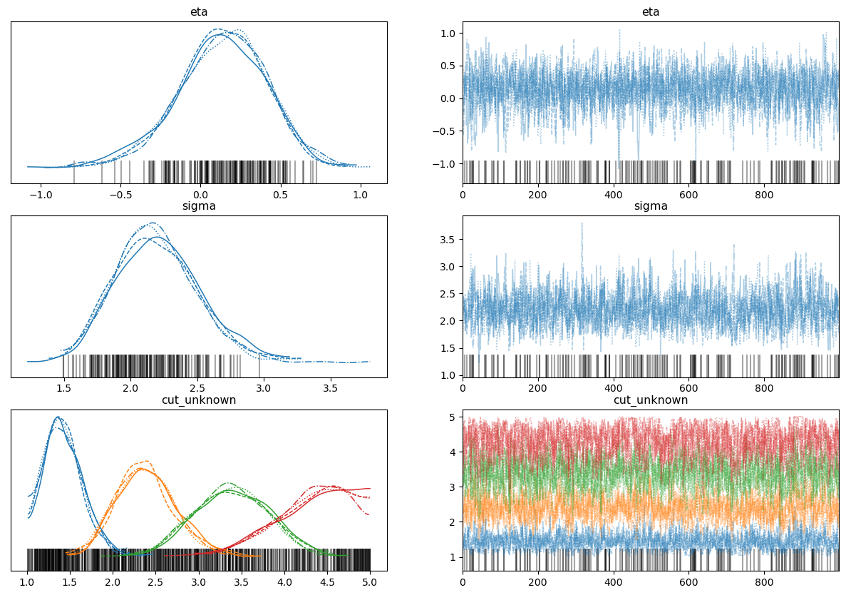
I’ve been using the following parameterisation (forgive hard-coding of values) which results in relatively sensible estimates (but not of the mean), but with severe divergences, and requires starting values to not crash:

df = pd.read_csv('OrdinalProbitData-1grp-1.csv')

with pm.Model() as model2:

    eta = pm.Normal('eta',  mu=3, sigma=2)
    sigma = pm.HalfNormal('sigma', 1)

    cutpoints = at.concatenate([
            [0.5],
            pm.Uniform('cut_unknown', lower=1, upper=5, shape=4),
            [5.5]
    ])

    pm.OrderedProbit('y' cutpoints=cutpoints, eta=eta, sigma=sigma,
                     compute_p=False, observed=df.Y.values-1)

    trace = pm.sample(tune=5000, initvals={'cut_unknown': [1.5, 2.5, 3.5, 4.5]})

az.plot_trace(trace, figsize=(15, 10))

Divergences aside, these look reasonable for the cutpoints and sigma, but not really for the mean (eta). The posterior predictive also looks very reasonable here. I know the cutpoints need to be ordered; I’ve tried transforming the Uniform prior in the code above using distributions.transforms.ordered and that actually increases the number of divergences!

image

Using the constrainedUniform implementation from @drbenvincent’s notebooks, the divergences disappear as stated, but now the estimates of the mean and scale are very different from 1 and 2.5, and the cutpoints are no longer on the scale of the responses:

def constrainedUniform(N, min=0, max=1):
    return pm.Deterministic('theta',
                            at.concatenate([
                                np.ones(1)*min,
                                at.extra_ops.cumsum(pm.Dirichlet("theta_unknown", 
                                                                 a=np.ones(N - 2))) * (min+(max-min))
                            ]), dims='cutpoints')

coords = {'cutpoints': np.arange(6)}

with pm.Model(coords=coords) as model2:

    eta = pm.Normal("eta", mu=3, sigma=2)
    sigma = pm.HalfNormal('sigma', 1)

    cutpoints = constrainedUniform(7)

    pm.OrderedProbit("y", cutpoints=cutpoints, eta=eta, sigma=sigma,
                     compute_p=False, observed=df.Y.values-1)

    trace = pm.sample(tune=5000)

az.plot_trace(trace)

image

I’m probably missing something fundamental here about OrderedProbit, but I’m not sure why having the cutpoints on their cumulative probability scale helps so much, or why the eta and sigma parameters never seem to quite reflect the values stated in DBDA2.

Any pointers are massively appreciated from this struggling Bayesian :pray:t2:

Sorry for the delayed response on this… we’re in the busy pre-xmas break period. How’s the progress going with this? I know I gave some input in another location, but this kind of thing is best suited to here on Discourse.

Hey @drbenvincent no problem. I’ve been working on this on and off, and not getting too much further along!

My main confusion stems from what appears to be a reasonable model causing massive divergences. I modified the above model a little to try to approximate the Kruschke version, with an ordered-normal prior on the cutpoints and pinning the left and right extreme cuts:

with pm.Model() as try_again:
    
    # Priors for mu and sigma
    μ = pm.Normal('μ', mu=3, sigma=3)
    σ = pm.HalfNormal('σ', sigma=3)
    
    # Cutpoints
    cutpts = at.concatenate([
        np.ones(1)*.5,
        pm.Normal('theta', mu=[1, 2, 3, 4], sigma=3, shape=4,
                  transform=pm.distributions.transforms.ordered),
        np.ones(1)*5.5
    ])
    
    cuts = pm.Deterministic('cuts', cutpts)
    
    # Ordered
    pm.OrderedProbit('ll', eta=μ, sigma=σ, cutpoints=cuts, compute_p=False, observed=df.Y.values-1)
    
    trace = pm.sample(tune=2000)

This samples, seems to converge, but has lots of divergences and again does not retrieve the mean of 1.

You mention on the discussion that the min and max arguments can perhaps shift the bounds of the constrained uniform - I will try that.

I guess my question at this point is more about the practicalities of this, just trying to grasp this stuff. The constrained uniform approach explicitly sets the first cutpoint to be zero, and then implicitly the final cutpoint is one. The cumulative sum guarantees the ordering of each cutpoint - but why does this sample so well compared to a transformed normal version? The cumulative sum on the Dirichlet is very neat but unintuitive to me. I wondered too about the “dims” argument in the call to pm.Deterministic - it seems essential but I can’t figure out why the need to do that.

Sorry for the mass of comments here and thank you!

So I am not an expert on inner workings of the sampler, but I believe it basically comes down to gradients. Old sampling algorithms evaluate the log probability of any given set of parameters given the data and model. Newer algorithms require not just an evaluation of the log probability, but also of the gradient. That gives the sampler information about which directions in (high dimensional) parameter space lead to what changes in the log probability.

The reason why we can’t just write arbitrarily complex python code is that while it would provide the logp, it wouldn’t provide the gradient information. This is why we shift over to using Aesara (now PyTensor) or JAX or similar libraries… they provide gradient information that the sampler needs.

So getting to your question… I guess the answer is that while the ordered transformation ‘works’, it is perhaps hard to correctly do all the autodifferentiation etc to get the gradients. But by taking a slightly loner route around (code wise) with the Dirichlet and the cumulative sum, I assume that these operations are much more ‘friendly’ in terms of calculating the gradient information.

But I’m tagging @lucianopaz and @ricardoV94 to see if I’ve made any major errors in my explanation.

Let me know how it goes. I am away from my textbooks now so I can’t check exactly what Kruschke’s results are. But I think there has been enough interest in ordinal regression models at this point for some of us to put together some definitive PyMC resources.

Tagging @bwengals and @tcapretto just to flag this up. Not sure who it should be, but I think it would be great if we/someone puts together some more definitive resources on ordinal regression for the community. What do you think?

Thank you for all the tips here @drbenvincent. That makes sense - I’m comfortable with some simple re-parameterisations to please the sampler, but the Dirichlet approach was so far outside my intuition I couldn’t grasp it at all! It does make some more sense now and altering the min and max arguments makes things a bit clearer. I only tried quickly, but on the Kruschke data, fixing the cutpoints to the suggested yielded very similar estimates for the cutpoints and scale, but the mean was still slightly off.

I’m likely not going to be much use but I’m happy to contribute or test any ordinal regression resources. Would be amazing to see this woven into bambi one day in the future!

Thank you and happy holidays!

1 Like

Would like to tag @cmgoold too, I know he’s worked on a lot of ordinal regression models and their variations.

Thanks @bwengals!

I threw the data into the model I mentioned here and here are the results:

               mean    sd  hdi_3%  hdi_97%  ess_bulk  r_hat
mu             1.05  0.30    0.49     1.60    3737.0    1.0
sigma          2.06  0.34    1.49     2.74    2769.0    1.0
theta_star[0]  1.50  0.00    1.50     1.50    4000.0    NaN
theta_star[1]  2.32  0.17    2.02     2.66    4432.0    1.0
theta_star[2]  3.16  0.26    2.67     3.65    3590.0    1.0
theta_star[3]  4.01  0.32    3.42     4.63    3509.0    1.0
theta_star[4]  4.81  0.34    4.16     5.41    3712.0    1.0
theta_star[5]  5.64  0.29    5.10     6.16    4457.0    1.0
theta_star[6]  6.50  0.00    6.50     6.50    3662.0    1.0

Looking at the Kruschke results, the sigma mean is a little low, but then again the priors are not exactly the same. The model runs cleanly in 20-40 seconds depending on the priors used.

I haven’t looked at the ConstrainedUniform implementation in depth, but there are differences in how my model and the model above is setting the limits to the cutpoints, and that’s going to influence the mean and sd estimates. I can look further into the differences too.

1 Like

Thanks @bwengals and @cmgoold! I’m a bit more experienced now with the general idea of the Dirichlet but this is good to see!

In a recent post here @tcapretto indicated PyMC v5 has fixed and updated the ordered transform for pm.Normal. I’ve been a bit busy working on that project but the code I imagine is the same; I wonder now if v5 would work with a Normal prior on the cutpoints now?

I guess the issue is that there is a need to fix the top and bottom cutpoints to constants, and the question is what (necessarily) multivariate prior sits between those constants and how this affects sampling/inferences! I’ll try to find some time to explore this and report back.