Symbolic gradient of GP posterior predictions

Is there a way to use Pytensor to calculate the symbolic gradient of the GP posterior mean (and possibly variance) with respect to the data domain? I’m trying to use pymc’s Marginal GP for (batched, offline) Bayesian Optimization of (biological) field experiments. I’m using a (generally isotropic) Matern 5/2 or 3/2 or ExpQuad kernel across 2-6 input dimensions, one output, and finding the MAP of the GP hyperparameters. Maximizing the acquisition function (generally Expected Improvement) would be much faster with access to the gradients of the mean and variance. Is this possible using pytensor.gradient? I’m not sure how to set that up to calculate the gradient at a given point in the input domain.

As a straightforward example, how would one find the gradient of this model: Marginal Likelihood Implementation — PyMC example gallery

1 Like

CC @aseyboldt @bwengals

Took a try at this, but I hope that @ricardoV94 or @aseyboldt would be able to take a look at this and show the best way to implement this.

So taking the model from the example you linked:

with pm.Model() as model:
    ell = pm.InverseGamma("ell", mu=1.0, sigma=0.6)
    eta = pm.Exponential("eta", scale=3.0)

    cov = eta**2 * pm.gp.cov.Matern52(1, ls=ell)
    gp = pm.gp.Marginal(cov_func=cov)

    sigma = pm.HalfCauchy("sigma", beta=5)
    y_ = gp.marginal_likelihood("y", X=X, y=y, sigma=sigma)

    marginal_post = pm.sample(draws=100, tune=300)

And then, you can calculate the symbolic mean and var of the predictions using ._predict_at,

# set symbolic input for new X locations
X_new = pt.tensor(dtype='float64', shape=(5, 1), name='X_new')

# take one point from the trace (or use the MAP estimate)
point = marginal_post.posterior.isel(draw=0, chain=0)

# calculate predictive mean and sd
with model:
    mu, var = gp._predict_at(
        X_new, diag=True
    )
    sd = np.sqrt(var)

# take one element of mu only because the `cost` input for `pt.grad`
# must be scalar (is it possible to vectorize this?)
grad = pt.grad(mu[1], wrt=X_new)
grad.eval({X_new: np.linspace(11, 12, 5)[:, None]})

gives

array([[ 0.        ],
       [-0.47514555],
       [ 0.        ],
       [ 0.        ],
       [ 0.        ]])
2 Likes

Answering the comment, probably yes with pt.vectorize

I’m not sure I understand the question correctly, please correct me if I misunderstood something.

You want to compute the gradient a posterior estimate of a parameter with respect to the x-positions where a gp was evaluated?

So for instance we have the following gp:

import pymc as pm
import pytensor.tensor as pt
import numpy as np
import matplotlib.pyplot as plt

np.random.seed(2)

n = 10
X = np.linspace(0, 10, n)

ell_true = 5.0
eta_true = 8.0
cov_func = eta_true**2 * pm.gp.cov.Matern52(1, ell_true)

mean_func = pm.gp.mean.Zero()

f_true = np.random.multivariate_normal(
    mean_func(X[:, None]).eval(), cov_func(X[:, None]).eval() + 1e-8 * np.eye(n), 1
).flatten()

sigma_true = 0.02
y = f_true + sigma_true * np.random.randn(n)

plt.plot(X, y)

image

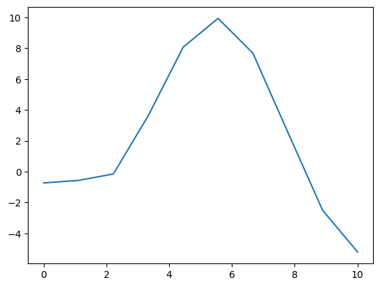
We can then model this to get a posterior over the mean of the gp:

with pm.Model(coords={"x_dim": X}) as model:
    ell = pm.InverseGamma("ell", mu=1.0, sigma=0.6)
    eta = pm.Exponential("eta", scale=3.0)

    cov = eta**2 * pm.gp.cov.Matern52(1, ls=ell)
    gp = pm.gp.Marginal(cov_func=cov)

    sigma = pm.HalfCauchy("sigma", beta=5)
    
    X = pm.Data("X_data", X)
    y = pm.Data("y_data", y)
    
    y_ = gp.marginal_likelihood("y", X=X[:, None], y=y, sigma=sigma)

    mu, var = gp._predict_at(
        X[:, None], diag=True
    )
    sd = np.sqrt(var)

    gp_mu = pm.Deterministic("gp_mu", mu.mean())

And you would now like to know what the gradient of gp_mu.mean(["draw", "chain"]) is with respect to X?

We can use a nice property of the posterior distribution. If we have any well behaved function f(\theta, \eta) where \theta are the parameters of the model and \eta are any other hyperparameters, then we can compute derivatives of F(\eta) = \int P(\theta|y, \eta) f(\theta, \eta) d\theta with

\frac{dF}{d\eta} = \int P(\theta|y, \eta) \left[\frac{df(\theta, \eta)}{d\eta} + (f(\theta, \eta) - F(\eta)) \frac{d}{d\eta}\log(P(y|\theta, \eta)) \right]

And given samples from P(\theta|y, \eta) we can approximate both integrals using their monte-carlo estimate (ie just the mean over the draws).

In this case we want \eta = X and f(\theta, \eta) = \text{gp_mu}, so that F(\eta) is just the posterior mean of gp_mu.

We can then compute the gradient as follows (adding to the model above):

with pm.Model(coords={"x_dim": X}) as model:
    logp = model.logp()
    # The derivatives in the integral above
    pm.Deterministic("dlogp_dx", pt.grad(logp, X), dims=("x_dim",))
    pm.Deterministic("dmu_dx", pt.grad(gp_mu, X), dims=("x_dim",))
    
    tr = pm.sample(nuts_sampler="numpyro")

And to get the gradient:

f = tr.posterior.gp_mu
F = f.mean(["draw", "chain"])
(tr.posterior.dmu_dx + (f - F) * tr.posterior.dlogp_dx).mean(["draw", "chain"]).plot()

image

Which I think makes sense? For instance if the first or second x-value was a bit smaller or bigger, our estimate for the mean wouldn’t change much. But if the third x-value was bigger, then the peak would start later, and be therefore smaller, meaning the mean of the GP should be smaller.

If you don’t want to compute the full posterior but only the MAP, you can use the implicit function theorem to get the derivatives of the MAP-estimates. The easiest way to do that in practice is probably to export the model to jax, and then use optjax or optimistix to compute the MAP, those implement those derivatives already.

I hope this wasn’t too much in one go with too little explanation, feel free to ask if something doesn’t make sense to you.

1 Like

Thanks for your help everyone! @bwengals’ solution is what I was looking for: given a single X_new point, calculate the gradient of the posterior mean at that point. Rewritten slightly:

with model:
    MAP = pm.find_MAP()

X_new = np.linspace(0, 20, 600)[:, None]

import pytensor
import pytensor.tensor as pt

# set symbolic input for new X locations
X_star = pt.tensor(dtype='float64', shape=(1,1), name='X_new')

# calculate predictive mean and sd
with model:
    mu, var = gp._predict_at(
        X_star, diag=True
    )
    sd = np.sqrt(var)

dμdX = pt.grad(mu[0], wrt=X_star)
dμdX = pytensor.function([X_star], dμdX)

grad_μ = np.vstack([dμdX(X_[:,None]) for X_ in X_new])

plt.plot(X_new, grad_μ)

Which looks like you’d expect!

@ricardoV94 , it would be nice to be able to vectorize this (although my primary use-case will be scalar, for maximization). I don’t see a vectorize module/function within pytensor. Maybe scan? But is scan true vectorization, or just a graph representation of a for loop?

@aseyboldt, that went beyond what I needed, but it’s interesting to see how you could get access to the gradient of the GP mean within the model! As a slight aside, do you think you could use this approach to constrain the GP, for instance to ensure the GP has a strictly-positive derivative? You’re right that, if all I’m interested in is using the MAP, jax is probably a more convenient way to get symbolic gradients. I was hoping to avoid rewriting my model construction in GPJax if possible, but might eventually anyways.

1 Like

I don’t think you’d need to rewrite your model. You can take the PyMC model’s logp, convert it to a JAX function, then do whatever you want from there. This is what we do when we access the numpyro/blackjax samplers, for example. See here.

1 Like

Regarding vectorize, our docs are lagging a bit behind, it’s defined here: pytensor/pytensor/tensor/functional.py at 75a9fd2ace49610095fb82548b3de1a80f3a6277 · pymc-devs/pytensor · GitHub

1 Like