I have a problem in which I want to infer the correlation structure of some data. I am using the LKJ distribution and I want to retrieve the posterior distribution of etas. However, the results always generate the same distribution. I have tried with many examples of generated data and I do not know what I am missing. For example, assuming that the correlation matrix is a Identity matrix, I am generating the most extreme case, where eta should tend to infinity. However, I find:
import pymc3 as pm
import numpy as np

D=10
y = np.identity(D)

il1 = np.triu_indices(D,1) #LKJCorr reads only the upper tri part of the matrix
obs = y[il1] # Taking upper tri of matrix

with pm.Model() as model:
    h_eta = pm.Uniform('eta', lower=0.00001, upper=3000)
    packed_L = pm.LKJCorr('obs_cov',eta=h_eta, n=D, observed=obs)
    #step = pm.Metropolis()
    trace = pm.sample(9000,njobs=2,nuts_kwargs=dict(target_accept=.95))

pm.traceplot(trace)
I’ve never really understood what eta does (I think I observed that my results were independent of the value I set there). So I’ve taken the occasion and tried to play around with this:
I can reproduce this with the code provided by @monteiro.
I also fiddled with the prior (pm.Bound(pm.HalfFlat, lower=0.00001), then with upper bound > 3000) but still retrieve lower boundary eta
bounding eta to >1 makes it still converge to minimal values just above one (I thought \eta \approx \epsilon might be a lokal minimum when cutting off infinity for numeric reasons)
When using an old example by Austin Rochford, which attaches a multivariate block of observations to the prior instead of just fitting the correlation matrix, eta (he called it nu) also takes very small values in posterior. test_eta2.py (1.4 KB) When leaving eta flexible, sampling is also not exactly fluent there, slowing down drastically at times, and chains fail late on. EDIT: file contained mistake, new try: test_eta2.py (1.5 KB) still a small eta.
Note that this last case could be also done with LKJCholeskyCov, which also has an eta parameter. EDIT: when using this prior, the sampling is much faster test_eta3.py (1.8 KB). However, eta still remains close to zero.
The documentation in pymc3/distributions/multivariate says:
For eta → oo the LKJ prior approaches the identity matrix.
So eta always tends to have a very small magnitude posterior. How come?
My understanding of the pymc3 code is not advanced enough to tell you what’s going on behind the scenes.
I guess this is something for the developers! Thanks for clearing it up.
Hmm I dont completely understand why as well. I doubt checked the LKJCorr logp implementation today and they are correct. For what is worth, I try to model the marginal density directly using what described in the LKJ paper:
As in case of the vine method, every off-diagonal element of the random correlation matrix R has a marginal density Beta(η+[d−2]/2,η+[d−2]/2) on (−1,1).
with pm.Model() as model:
    h_eta = pm.Uniform('eta', lower=0.00001, upper=3000, testval=1000.)
    packed_L = pm.Beta('obs_cov', alpha=h_eta+(D-2)/2, beta=h_eta+(D-2)/2, observed=obs/2+.5)
    trace = pm.sample()
The resulting eta is as expected concentrated around the upper limit.
So my guess this might be something to do with the normalizing constant. In another word, while \eta \to \infty you get identity matrix when generate from LKJCorr, the reverse is not true as the posterior of p(\eta \mid observed) does not normalized the same way. Looking at the logp implementation, as logdet(observed) is zero, what is left is the normalizing constant. So have a look at how it changes using something like Wrong logp in LKJ prior · Issue #1042 · pymc-devs/pymc · GitHub would give you some intuition.
Thank you @falk and @junpenglao.
In the short term I will use the alternative parametrization. Quick question, though: is there a specific reason for observed=obs/2+.5? I could not find on the LKJ paper.
The marginal is defined on (-1, 1) but Beta distribution is defined on (0, 1), this is to put the observed value from (-1, 1) to (0, 1).
Now you mentioned about it, I should account for the jacobian of the transformation…
So, assuming the correlation matrix R= 2u − 1, where u ∼ Beta(β, β), and β = η + (d − 2)/2.
The final script would be:
import pymc3 as pm
import numpy as np

D=10
y = np.identity(D)

il1 = np.triu_indices(D,1) #LKJCorr reads only the upper tri part of the matrix
obs = y[il1] # Taking upper tri of matrix
obs=(obs+1)/2

with pm.Model() as model:
    h_eta = pm.Uniform('eta', lower=0.00001, upper=3000, testval=1000.)
    R = pm.Beta('R', alpha=h_eta+(D-2)/2, beta=h_eta+(D-2)/2, observed=obs)
    trace = pm.sample()

pm.traceplot(trace)
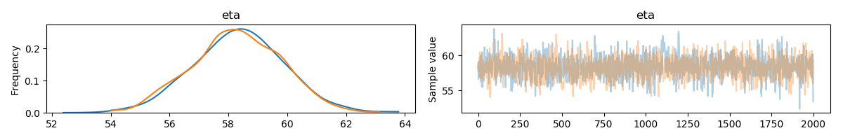
To make sure, we may generate known \eta and check the results