Why doesn't this pymc3 model show shrinkage?

[James_Vanneman]

I’m trying to understand shrinkage and I’ve built a really simple model that I thought should show shrinkage between the two p parameters of the binomial distribution:

with pm.Model() as model:
    alpha = pm.HalfNormal('alpha', 3)
    beta = pm.HalfNormal('beta', 3)
    ps = pm.Beta('ps', alpha=alpha, beta=beta, shape=2)
    pm.Binomial('obs', p=ps, n=[6, 125], observed=[1, 110])

    traces = pm.sample(3000, cores=2, tune=500)

I assumed since both ps[0] and ps[1] share a higher level distribution, the significantly more number of draws from ps[1] would influence the probability of ps[0], but based on the posterior estimates, it doesn’t look like it has any effect:

[AlexAndorra]

Hi James,
I think you need to check the group mean to understand how shrinkage works in your model. But in your parametrization it’s not clear to me what the group mean is – probably a combination of alpha and beta. I think I’d use another parametrization to have a clear group mean. Something like:

with pm.Model() as model:
    a = pm.Normal('a', 0., 1.) # group mean
    sigma = pm.Exponential('sigma', 1.) # determines amount of shrinkage

    a_cluster = pm.Normal('a_cluster', a, sigma, shape=2)
    p = pm.math.invlogit(a_cluster[cluster_id])

    pm.Binomial('obs', p=p, n=[6, 125], observed=[1, 110])

That way, it’s clear that a is the group mean, which individual-level parameters are shrunk to, and sigma is the amount of shrinkage (the smaller, the more similar the clusters, so the more shrinkage).

That being said, I think your model does shrink towards the group mean: the blue distribution is centered around 0.3, while the observed data are 0.16 (1/6). Of course, the orange one is centered on the observed data and much less wide because there is a lot more data to infer it.

If you’re looking for ressources, there is a whole chapter on hierarchical models and shrinkage in McElreath’s Rethinking – here is the port to PyMC (we’re working on porting the 2nd ed. but you’ll have to wait a bit ). And these models are the topic of the last episode of my podcast, with Thomas Wiecki.
Hope this helps

[James_Vanneman]

That makes a lot of sense, being able to reason about your group mean and the level of shrinkage seems like a clear win for that parameterization. With that parameterization, the models issues a few warnings:

Auto-assigning NUTS sampler...
Initializing NUTS using jitter+adapt_diag...
Multiprocess sampling (2 chains in 2 jobs)
NUTS: [a_cluster, sigma, a]
Sampling 2 chains, 9 divergences: 100%|██████████| 5000/5000 [00:02<00:00, 2024.95draws/s]
There were 2 divergences after tuning. Increase `target_accept` or reparameterize.
There were 7 divergences after tuning. Increase `target_accept` or reparameterize.

What changes if any would you make with these warnings? Feel free to link to some more great resources if anything comes to mind.

I actually already ordered Rethinking(second edition), I’ll keep an eye out for your PyMC port and I’ll definitely check out your podcast . Thanks for you help!

[nkaimcaudle]

You need to be careful with divergences, the first thing to check is if they are clustering in some area of the parameter space. Using ArviZ we can get a pairs plot which will easily highlight the divergent parameter sets.

Here you can see they are mostly spread out, so the next step would be to adjust target_accept in pm.sample()

trace = pm.sample(target_accept=0.95)

The default value is 0.8, if PyMC gives you that warning then typical values to try are 0.90, 0.95 and 0.99.

Here is a very good resource I find myself looking at often for many different modelling issues

Cookbook — Bayesian Modelling with PyMC3

If you want to get deeper into the issues with divergences and how they impact modelling then there is a very indepth blog written by the Stan community, a similar C based bayesian probabalistic language
https://betanalpha.github.io/assets/case_studies/divergences_and_bias.html

[James_Vanneman]

Those are great resources, thank you. Read through a lot of that and here’s how I proceeded. My first attempt was to do what you suggested, I tried target_accept of 0.9, 0.95 and 0.99. At all of those values, I would non-deterministically get rid of divergences on some runs, but other runs would have between 1-12 divergences. At a value of 0.995, it completely got rid of the divergences. I wanted to explore other options, and I’m curious if this hybrid approach has any merits. I’m also wondering if a target_accept of 0.995 has any negative downsides that might prevent you from wanting to use that value(high auto-correlation, slow convergence?). It also seems very wrong to rely on a model that sometimes will have divergences and sometimes will not.

With a target_accept of 0.95:

with pm.Model() as model:
    a = pm.Normal('a', 0., 1.)
    sigma = pm.Exponential('sigma', 1.)
    a_cluster = pm.Normal('a_cluster', mu=a, sigma=sigma, shape=2)
    p = pm.math.invlogit(a_cluster[[0, 1]])
    pm.Binomial('obs', p=p, n=[6, 125], observed=[1, 110])
    traces = pm.sample(2000, cores=4, target_accept=0.95)

Auto-assigning NUTS sampler...
Initializing NUTS using jitter+adapt_diag...
Multiprocess sampling (4 chains in 4 jobs)
NUTS: [a_cluster, sigma, a]
Sampling 4 chains, 11 divergences: 100%|██████████| 10000/10000 [00:03<00:00, 3070.63draws/s]
There were 4 divergences after tuning. Increase `target_accept` or reparameterize.
There was 1 divergence after tuning. Increase `target_accept` or reparameterize.
There were 5 divergences after tuning. Increase `target_accept` or reparameterize.
There was 1 divergence after tuning. Increase `target_accept` or reparameterize.

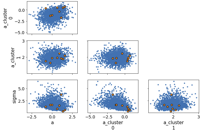
Looking at the pairplot of divergences:

pm.pairplot(traces,  divergences=True)

It appears that more divergences are cluster in the corner. I looked at the pairplot of sigma and individual group mean.

x = pd.Series(traces['a_cluster'][:, 0], name='a_cluster')
y = pd.Series(traces['sigma'], name='sigma')

sns.jointplot(x, y, ylim=(0, 2));

This shows a “funnel” shape, which makes sense because as the group sigma gets smaller, it constrains the possible values of the group mean. The downside of this is that it can make it hard for the sampler to efficiently explore the space of lower sigmas. One of the suggestions you linked to talked about using an off-centered reparameterization, so I changed my code to:

with pm.Model() as model:
    a = pm.Normal('a', 0., 1.) # group mean
    sigma = pm.Exponential('sigma', 1.) # determines amount of shrinkage
    
    a_offset = pm.Normal('a_offset', mu=0, sd=1, shape=2)
    a_cluster = pm.Deterministic('a_cluster', a+a_offset*sigma)
    p = pm.math.invlogit(a_cluster[[0, 1]])

    pm.Binomial('obs', p=p, n=[6, 125], observed=[1, 110])
    traces = pm.sample(2000, cores=4, target_accept=0.95)

Which significantly reduced the number of divergences(on some runs I would still get 1 or 2). A target_accept of 0.99 completely removed divergences with this parameterization. A pair plot of the offset and sigma show they’re uncorrelated which (I think) makes it easier for the sampler to explore the space:

x = pd.Series(traces['a_offset'][:, 0], name='a_cluster')
y = pd.Series(traces['sigma'], name='sigma')

sns.jointplot(x, y, ylim=(0, 2));

[nkaimcaudle]

Your new model parameterisation is called non-centered and is generally more robust, though not always as pointed out in Statistical Rethinking.

A higher target_accept is slower to sample but I am not sure if there are other possible disadvantages, would need someone with more expertise to chime in.

[AlexAndorra]

Well done on this workflow James
Regarding target_accept, it does make sampling slower, so if your model was already slow, it could be a problem. Here it doesn’t seem to be the case. But as you said, you have to remain vigilant: if the model seems unstable and regularly shows divergences, then there could be a problem with your model itself. Here, I think you found it: the group sigma was very close to zero, so you needed the non-centered parametrization.

A couple more observations:

• The priors I used for sigma and, notably, a are not tailored to your model. Doing prior predictive checks could help your model sample better.
• I’m guessing you’re using toy data, but there are only a few of them, and only two clusters – at the group level, this means you’re trying to estimate a standard deviation (sigma) with only two data points (the clusters). This is of course a problem; you usually need at least 15-20 clusters I’d say.
• Taking more tuning samples would probably help the sampler. A good default for most simple models is pm.sample(1000, tune=2000). Most people take more tuned samples than tuning samples, but in the Bayesian framework I’d say the latter are more important than the former.

Hope this helps, and congrats again on making your model run