I noticed the chart pictured below from the DPMM example doesn’t seem to be showing “normal” components correctly.
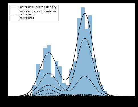
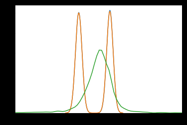
In the previous iteration of the example, the syntax was different for defining the model, but it produced what I believe is the correct chart/components (pictured below)
It’s clear to see that the “components” in above chart aren’t normally distributed, but bimodal. The below chart has correct normal components

Am I misunderstanding something about the output of DPMMs? Shouldn’t the components reflect the type of the base distribution?
If I’m correct, and there’s a problem with the exmaple, how can the correct components be obtained from the new DPMM syntax?
Seems there are some label switching in the new figure - we should rerun the notebook and check the inference more carefully.
1 Like
When I run the notebook NUTS doesn’t converge.
Some of the largest weights have gelman-rubin statistic of >3
Should I try to identify the label switching and manually fix it, or do you suspect there is a problem with the implementation in the new notebook causing this? I’m curious as to why the older syntax works correctly, or perhaps it’s the use of the metropolis and categorical steps in the older one.
Here’s a distplot of 2 of the ‘mu’ traces, showing bimodality:
It almost looks like sign-switching, but it’s not exactly symmetrical about 0
And these are the first 3 ‘w’:

It seems the label switching only occurs between chains, not within.
Sampling a single chain fixed the problem for me

Enforcing an “ordered” transform on “mu” also works, but I haven’t let it run enough samples yet, as it takes much longer.
mu = pm.Normal(‘mu’, 0, tau=lambda_ * tau, shape=K,
transform=pm.distributions.transforms.Ordered(), testval=np.linspace(-1, 1, K))

ADVI wasn’t working, even with the Ordered transform, etc.
Using the “SignFlipMeanFieldGroup” from the “Unique Solution for bPCA” thread allowed ADVI to infer normal components (see code below)

from pymc3.variational import approximations
from pymc3.variational.opvi import Group, node_property
import theano.tensor as tt
import theano

    @Group.register
    class SignFlipMeanFieldGroup(approximations.MeanFieldGroup):
        __param_spec__ = dict(smu=('d', ), rho=('d', ))
        short_name = 'signflip_mean_field'
        alias_names = frozenset(['sfmf'])

        @node_property
        def mean(self):
            return self.params_dict['smu']

        def create_shared_params(self, start=None):

            if start is None:
                start = self.model.test_point
            else:
                start_ = start.copy()
                update_start_vals(start_, self.model.test_point, self.model)
                start = start_

            if self.batched:
                start = start[self.group[0].name][0]

            else:
                start = self.bij.map(start)

            rho = np.zeros((self.ddim,))

            if self.batched:
                start = np.tile(start, (self.bdim, 1))
                rho = np.tile(rho, (self.bdim, 1))

            return {'smu': theano.shared(
                        pm.floatX(start), 'smu'),
                    'rho': theano.shared(
                        pm.floatX(rho), 'rho')}

        @node_property
        def symbolic_logq_not_scaled(self):
            z = self.symbolic_random

            logq = - tt.log(2.) + tt.log(
                             tt.exp(pm.Normal.dist(self.mean, self.std).logp(z)) + \
                             tt.exp(pm.Normal.dist(-self.mean, self.std).logp(z)))

            return logq.sum(range(1, z.ndim))
I used the reduce_rate learning_rate schedule from the LDA AEVB example which got ADVI to converge much faster to the results obtained from NUTS.
with model:
    symmetric_group = pm.Group([mu], vfam='sfmf')
    other_group = pm.Group(None, vfam='mf')
    approx = pm.Approximation([symmetric_group, other_group])
    inference = pm.KLqp(approx)

η = .001
s = theano.shared(η)
def reduce_rate(a, h, i):
    val=η/((i/len(old_faithful_df))+1)**.7
    s.set_value(val)


inference.fit(20000, obj_optimizer=pm.sgd(learning_rate=s), callbacks=[reduce_rate])

Yeah you need to kinda lie to yourself and sample only one mode… And there are efforts to improve the sampling of that notebook but we never really got it fix… https://github.com/pymc-devs/pymc3/pull/2956