Hi all,
Possibly related to this thread but for the moment stay with me.
I’ve tried to add as much code and explanation as possible. Sorry if this is overkill.
I am trying to use pymc in a polynomial regression model up to the 5th order. The reason for using pymc over bambi is the regression will happen within a calculation process (matrix inversion) that I believe babmi would not be able to handle. That’s a battle for another day I suspect…
For now, I am considering a toy problem.
y = 5t^2 + 4t^4 + 3t^3 + 2t^2 + t + 1.5
for which the coefficients
\beta = [5, 4, 3, 2, 1]
Intercept = 1.5
would be recovered.
I’ve been basing my approach on the Bambi example for Orthogonal Polynomial Regression. The formula for y above, with some additive noise (\sigma = 5) in the observation looks like this

code for the above is as follows:
true_intercept = 1.5
t = np.linspace(0, 2, 100)
x_true = 5*t**5 + 4*t**4 + 3*t**3 + 2*t**2 + t + true_intercept
noise = np.random.normal(0, 5, x_true.shape)
x_obs = x_true + noise
df_projectile = pd.DataFrame({"t": t, "x": x_obs, "x_true": x_true})
df_projectile = df_projectile[df_projectile["x"] >= 0] # can't go lower than ground = 0!

plt.scatter(df_projectile.t, df_projectile.x, label='Observed Displacement', color="C0")
plt.plot(df_projectile.t, df_projectile.x_true, label='True Function', color="C1")
plt.xlabel('Time (s)')
plt.ylabel('Displacement (m)')
plt.ylim(bottom=0)
plt.legend()
plt.show()
- Bambi Model
The Bambi model takes the following form
model_projectile_all_terms = bmb.Model("x ~ I(t**5) + I(t**4) + I(t**3)+ I(t**2) + t + 1", df_projectile)
fit_projectile_all_terms = model_projectile_all_terms.fit(idata_kwargs={"log_likelihood": True}, random_seed=SEED)
az.summary(fit_projectile_all_terms)

az.plot_posterior(
    fit_projectile_all_terms,
    ref_val=[5, 1.5, 5,4,3,2,1],
    hdi_prob=0.94  # 94% highest density interval
)
plt.tight_layout()
plt.show()
and produces the following posterior distributions. Although they engulf the ‘true’ values, the spread of possible values is huge in some cases.

- PYMC version with Q,R decomposition
Here, I try to repeat what I understand is going on under the hood with Bambi. This hinges on the Q,R decomposition which has been implemented (correctly - I hope) by mirroring the advice here
After a bit of tweaking with prior predictive checks to ensure the scale of predictions was acceptable

I get a similarly odd posertier - with very wide spread in distributions. See below.

here’s the code
""" try a QR decomposition in pymc """
# first standardise the predictor
mean = np.mean(t)
t_centered = t - mean

# Construct the design (Vandermonde) matrix: columns [1, x, x^2, x^3, x^4, x^5]
X = np.column_stack([np.ones_like(t), t, t**2, t**3, t**4, t**5])

# QR Decomposition of Design Matrix
Q, R = np.linalg.qr(X)
N = X.shape[0]

# Scaling as per advice
Q_star = Q * np.sqrt(N - 1)
R_star = R / np.sqrt(N - 1)

# Pre-compute the inverse of R* for recovering original coefficients later
R_star_inv = np.linalg.inv(R_star)

# PYMC MODEL

with pm.Model() as model:
    # Priors on the transformed coefficients (theta), one for each column of Q_star.
    theta = pm.Normal('theta', mu=0, sigma=20, shape=6)

    # Prior on observation noise (sigma)
    sigma = pm.HalfNormal('sigma', sigma=5)

    # Linear predictor in the orthogonalized space
    mu = pm.math.dot(Q_star, theta)

    # Likelihood
    y = pm.Normal('y', mu=mu, sigma=sigma, observed=observation)

    # Deterministically recover original coefficients: beta = R*^{-1} * theta
    original_coefs = pm.Deterministic('original_coefs', pm.math.dot(R_star_inv, theta))

   # SAMPLE!
    trace = pm.sample(draws=2000, tune=2000, chains=4, random_seed=42)

#PLOT
az.plot_posterior(
    trace,
    var_names=["original_coefs", "sigma"],
    ref_val=[1.5, 1,2,3,4,5, 5],
    hdi_prob=0.94  # 94% highest density interval
)
plt.tight_layout()
plt.show()
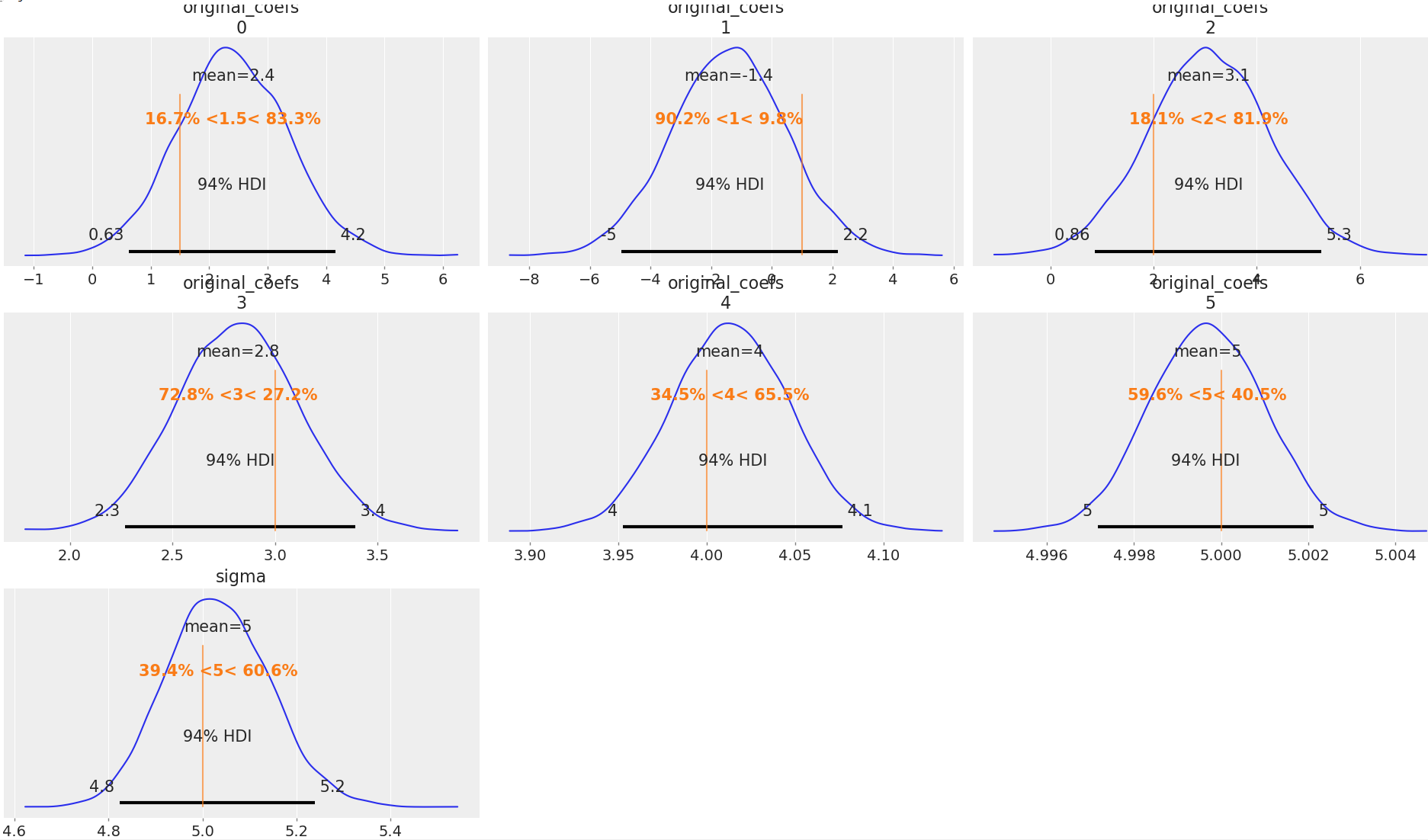
I also tried a simple, more direct route. No decomposition, just direct inference on each of the coefficients. Funnily enough, this was quite good.

code for the above plot
# try the pymc way
t_py = pt.as_tensor_variable(t)
observation = pt.as_tensor_variable(x_obs)

with pm.Model() as model:
    #beta coeff priors - directly estimated
    beta = pm.Normal("beta", mu = 2, sigma = 1.5, shape = 6)

    #noise
    sigma_noise = pm.HalfNormal("sigma_noise", sigma=5 )

    # likelihood
    x_pymc = beta[5] * t_py**5 + beta[4]*t_py**4 + beta[3]*t_py**3 + beta[2]*t_py**2 + beta[1]*t_py + beta[0]

    likelihood = pm.Normal("likelihood", mu=x_pymc, sigma = sigma_noise, observed=observation)

    # sample
    trace = pm.sample(
       draw = 2000,
        tune=2000,
        chains=4)

#PLOT
az.plot_posterior(
    trace,
    # var_names=["original_coefs"],
    ref_val=[1.5, 1,2,3,4,5, 5],
    hdi_prob=0.94  # 94% highest density interval
)
plt.tight_layout()
plt.show()
HELP NEEDED
Given the short story presented here, I wondered if any supportive souls could point out any inaccuracies/errors in my approach and recommend improvements. I am particularly keen to understand the issues around the QR decomposition aspect when executed in PYMC.
This is all quite unchartered territory for me, so any help, no matter how basic, would be great.
Side note: I did see in this paper that “The main problem is that QR decomposition is not unique”. Could this be a factor?
Thanks in advance