I am trying to tackle a problem where I have a set of low frequency time series that I want to disaggregate to high frequency using high frequency indicator variables.
I was wondering how I could model this as a bayesian problem such that I can get posterior distributions of the daily estimates.
I am an amateur, so detailed answers are welcome. Any pointers to example implementations will be super helpful.
I am the author of tsdisagg, a package for doing the “usual” methods (denton, denton-cholette, chow-lin, litterman).
Basically the difficultly in these methods is just setting up the problem. You need to decide if your variables are stocks or flows, and based on that, what kind of aggregation you need to do to go from high frequency to low frequency. Those decisions will determine a mapping from a (usually linear) high frequency estimate (just \mu_{hf} = X\beta, where X is a matrix of high-frequency indicator variables) back to the low frequency data, \mu_{lf} = CX, where C is the conversion matrix. After that, it’s just a simple linear regression, potentially with a special covariance matrix.
You can re-use the helper function from tsdisagg to set up a problem. Here is an example using the Swedish pharmaceutical sales dataset from Sax and Steiner 2013:
import pandas as pd
from tsdisagg.ts_disagg import build_conversion_matrix, prepare_input_dataframes

sales_a = pd.read_csv("https://raw.githubusercontent.com/jessegrabowski/tsdisagg/refs/heads/main/tests/data/sales_a.csv", index_col=0)
sales_a.index = pd.date_range(start="1975-01-01", freq="YS", periods=sales_a.shape[0])
sales_a.columns = ["sales"]

exports_q = pd.read_csv("https://raw.githubusercontent.com/jessegrabowski/tsdisagg/refs/heads/main/tests/data/exports_q.csv", index_col=0)
exports_q.index = pd.date_range(start="1972-01-01", freq="QS", periods=exports_q.shape[0])
exports_q.columns = ["exports"]

_, low_freq_df, high_freq_df, time_conversion_factor = prepare_input_dataframes(
    sales_a, exports_q.assign(intercept=1), target_freq=None, method='chow-lin'
)
C = build_conversion_matrix(low_freq_df, high_freq_df, time_conversion_factor, agg_func='sum')
prepare_input_dataframes matches up the two dataframes based on the frequencies on their DateTimeIndex. build_conversion_matrix builds the linear mapping from the high frequency data to low frequency data, based on the requested aggregation statistics. In this case, sales are a flow variable, so I’m using sum as the aggregation statistic. In this case, C has shape (36, 158), because there are 36 low-frequency observations (annual) and 158 high-frequency (quarterly). The structure of the matrix is such that for each year (row), the four quarters (columns) corresponding to that year have 1, and all other values are zero. Thus, C @ X adds the quarters back up to years.
Once you have this all set up, the pymc model is just a basic linear regression in the high frequency space, followed by a projection back to low-frequency space where the observed data lives:
import pymc as pm

coords={'feature': ['exports', 'intercept'],
        'high_freq_time': high_freq_df.index,
        'low_freq_time': low_freq_df.index}

with pm.Model(coords=coords) as simple_model:

    y = pm.Data('y', low_freq_df['yearly_sales'], dims=['low_freq_time'])
    X = pm.Data('X', high_freq_df, dims=['high_freq_time', 'feature'])

    beta = pm.Normal('beta', 0, 10, dims=['feature'])

    mu_quarterly_sales = pm.Deterministic('mu_quarterly_sales', X @ beta, dims=['high_freq_time'])
    mu_annual_sales = C @ mu_quarterly_sales

    sigma_sq = pm.Exponential('sigma_sq', 1)

    y_hat = pm.Normal('y_hat',
                      mu=mu_annual_sales,
                      sigma=pm.math.sqrt(sigma_sq),
                      observed=y, dims=['low_freq_time'])

    idata_1 = pm.sample()
Results:
                   mean     sd  hdi_3%  hdi_97%  mcse_mean  mcse_sd  ess_bulk  ess_tail  r_hat
beta[exports]     0.013  0.000   0.013    0.014      0.000    0.000    2122.0    2176.0    1.0
beta[intercept]  12.371  0.630  11.217   13.570      0.014    0.011    2141.0    2238.0    1.0
sigma_sq         78.777  6.083  67.520   90.354      0.125    0.094    2330.0    2420.0    1.0
Compared to the chow-lin method in tsdisagg:
Dependent Variable: yearly_sales
GLS Estimates using Chow-Lin's covariance matrix
N = 158		df = 154
Adj r2 = 0.9948

Variable             coef         sd err              t        P > |t|         [0.025         0.975]
----------------------------------------------------------------------------------------------------
exports            0.0134         0.0001        91.0941         0.0000         0.0131         0.0137
intercept         12.4089         1.2963         9.5724         0.0000         9.8480        14.9697

rho                0.0000
sigma.sq          98.8717
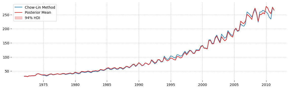
We can see that the estimates essentially agree 100%. The variance estimate is a bit different, this is likely the influence of the prior pulling the estimate down.
Plotting the two outputs shows the strong agreement in methods:
One problem with this plot is that I’m only plotting the posterior uncertainty, not the posterior predictive uncertainty. I think you could have a better plot by thinking about how to divide the estimated annual variance between the four quarters. I assume it would be something like the fourth-root of estimated variance, but I didn’t think about it carefully, nor did I try the exercise. If you choose to, you just need to set up a predictive model, giving mu_quarterly_sales and the scaled variance to a new pm.Normal, then call pm.sample_posterior_predictive.
I also did the exercise with full chow-lin covariance matrix, but it wasn’t very interesting. Full code is in this gist here.
Thanks a lot for the comprehensive response.
This is super helpful.
tsdisagg is a great reference.
I am actually trying to do something that has a layer of complexity over this. A hierarchical model that incorporates time series disaggregation.
As an example, consider that you have a hierarchical time series structure. Specifically, say you have energy demand on a monthly level at the state and county level.
You want to estimate daily energy demand per county and for the entire state. The catch is that you have high frequency indicators only for a subset of counties.
My current plan is to extend the approach you presented into a hiearchical framework.
You can have multiple observed variables in a model without issue. You could take the exact model I posted, then continue adding lines below the y_hat variable that use the latent mu_quarterly_sales time series however you please. You should keep the observed low frequency series though, so that the model has to take into account that the disaggregated time series has to plausibly generate that data (in addition to whatever your final data of interest are)