Behrens' Bayesian Learner Model : How to share parameters between steps?

Hi!

I am trying to implement Bayesian Learner Model of Tim Behrens. It’s a model like this:

CleanShot 2021-07-09 at 16.07.30@2x

Behrens infer some parameters in our brain changed over time.

y is the choice of subjects and r is the proportion if y == 1.

And the update rule of parameters follows the Bayesian rule like this:

\mathrm{p}\left(\mathrm{r}_{\mathrm{i}+1} \mid \mathrm{r}_{\mathrm{i}}, \mathrm{v}\right) \sim \beta\left(\mathrm{r}_{\mathrm{i}}, \mathrm{V}\right)

and

p\left(v_{i+1} \mid v_{i}, k\right) \sim N\left(v_{i}, K\right)

One could find out the definition of this model on pages 5-6 of this appendix.

I meet SamplingError over time. And the most confusing problem is how to share the parameters of multi RVs between steps.

Here is my newest code (So many thanks to @ricardoV94 ):

import pymc3 as pm
import theano.tensor as tt
import pandas as pd
import numpy as np
from scipy import stats

# Create the test data
p = np.repeat([.75, .75, .75, .25, .75, .25], 100)
env= stats.binom.rvs(1, p)

# Modeling
with pm.Model() as bayesian_lerner_model:
    k = pm.Normal("k", mu = 1, sigma = 1, testval = 0.6)
    k_ = pm.Deterministic('k_cap', pm.math.exp(k))
    v = pm.GaussianRandomWalk("v", mu = 0.7, sigma = k_, testval = 0.05, shape = len(env))
    v_ = pm.Deterministic('v_cap', pm.math.exp(v))

    r = []
    for ti in range(len(env)):
        if ti == 0:
            # Testvals are used to prevent -inf initial probability
            r.append(pm.Beta(f'r{ti}', 1, 1))
        else: 
            w = r[ti-1]
            k = 1 / v_[ti-1]
            r.append(pm.Beta(f'r{ti}', alpha=w*(k-2) + 1, beta=(1-w)*(k-2) + 1, testval = 0.5))

    r = pm.Deterministic('r', pm.math.stack(r))
    y = pm.Bernoulli("y", p = r, observed = env)
    
    trace = pm.sample(return_inferencedata=True)

As the comparison, Michael Waskom implements the model by Numpy. Here’s his code:

"""Python implementation of a Bayesian probabilistic learner.

This model was originally described in Behrens et al. Nat Neuro 2007.

The code here was adapted from the original C++ code provided by
Tim Behrens.

"""
class ProbabilityLearner(object):

    def __init__(self, p_step=.01, I_step=.1):

        # Set up the parameter grids
        p_grid = make_grid(.01, .99, p_step)
        self.p_grid = p_grid
        I_grid = make_grid(log(2), log(10000), I_step)
        self.I_grid = I_grid

        self._p_size = p_grid.size
        self._I_size = I_grid.size

        # Set up the transitional distribution on p
        joint_grid = np.meshgrid(p_grid, p_grid, I_grid, indexing="ij")
        p_trans = np.vectorize(p_trans_func)(*joint_grid)
        self._p_trans = p_trans / p_trans.sum(axis=0)

        # Initialize the learner and history
        self.reset()

    @property
    def p_hats(self):
        return np.atleast_1d(self._p_hats)

    @property
    def I_hats(self):
        return np.atleast_1d(self._I_hats)

    @property
    def data(self):
        return np.atleast_1d(self._data)

    def fit(self, data):
        """Fit the model to a sequence of Bernoulli observations."""
        if np.isscalar(data):
            data = [data]
        for y in data:
            self._update(y)
            pI = self.pI
            self.p_dists.append(pI.sum(axis=1))
            self.I_dists.append(pI.sum(axis=0))
            self._p_hats.append(np.sum(self.p_dists[-1] * self.p_grid))
            self._I_hats.append(np.sum(self.I_dists[-1] * self.I_grid))
            self._data.append(y)

    def _update(self, y):
        """Perform the Bayesian update for a trial based on y."""

        # Information leak (increase in the variance of the joint
        # distribution to reflect uncertainty of a new trial)
        # -------------------------------------------------------

        pI = self.pI

        # Multiply P(p_p+1 | p_i, I) by P(p_i, I) and
        # integrate out p_i, which gives P(p_i+1, I)

        # pI = (self._p_trans * pI).sum(axis=1)

        # Equivalent but twice as fast:
        pI = np.einsum("ijk,jk->ik", self._p_trans, pI)

        # Update P(p_i+1, I) based on the newly observed data
        # ----------------------------------------------------------

        likelihood = self.p_grid if y else 1 - self.p_grid
        pI *= likelihood[:, np.newaxis]

        # Normalize the new distribution
        # ------------------------------

        self.pI = pI / pI.sum()

def make_grid(start, stop, step):
    """Define an even grid over a parameter space."""
    count = (stop - start) / step + 1
    return np.linspace(start, stop, count)


def I_trans_func(I_p1, I, k):
    """I_p1 is normal with mean I and std dev k."""
    var = exp(k * 2)
    pdf = exp(-.5 * power(I - I_p1, 2) / var)
    pdf *= power(2 * pi * var, -0.5)
    return pdf


def p_trans_func(p_p1, p, I_p1):
    """p_p1 is beta with mean p and precision I_p1."""
    a = 1 + exp(I_p1) * p
    b = 1 + exp(I_p1) * (1 - p)

    if 0 < p_p1 < 1:
        logkerna = (a - 1) * log(p_p1)
        logkernb = (b - 1) * log(1 - p_p1)
        betaln_ab = gammaln(a) + gammaln(b) - gammaln(a + b)
        return exp(logkerna + logkernb - betaln_ab)
    else:
        return 0

As a newbie, I have no idea which part of my code is wrong. So I am looking forward to your help.
Thanks!
1 Like

Are you not getting invalid p values in that Bernoulli at the end, when using the cumsum? p must be between 0 and 1.

1 Like

Thank you for your help, here I print my r_rw by using tt.printing.Print() and find out many values in the list larger than 1.

I think this is why I get a -inf logp of y.

So I know the problem of my program. But I still have no idea how to track the dynamic change of p…

I misunderstood the concept of Beta random walk (or random walk I am not sure).

cumsum not a valid way to track the dynamic change of my RVs.

I am not familiar with beta random walks but maybe you can try a logistic random walk. Have a normal gaussian random walk and use the logistic transformation to get a p in the range 0-1.

Thanks for your idea @ricardoV94 and I will try it.

But the biggest question is how can I implement Behrens’ Model according his paper. Is there something wrong in his model?

And I still have no idea how to observe a volatile variable in my model. I am sure there are some leak in my knowledge. And I am reading your GitHub to get more information.

The appendix you linked to is a bit long. Could you point where the model you are trying to implement is actually specified?

Wow, thank you for your help! @ricardoV94

Behrens infer some parameters in our brain changed over time. He built a graph model like this:

CleanShot 2021-07-09 at 16.07.30@2x

y is the choice of subjects and r is the proportion if y == 1.

And the update rule of parameters follows the Bayesian rule like this:

\mathrm{p}\left(\mathrm{r}_{\mathrm{i}+1} \mid \mathrm{r}_{\mathrm{i}}, \mathrm{v}\right) \sim \beta\left(\mathrm{r}_{\mathrm{i}}, \mathrm{V}\right)

and

p\left(v_{i+1} \mid v_{i}, k\right) \sim N\left(v_{i}, K\right)

You could find out the definition of this model on page 5-6 of this appendix.

What confused me is the parameters in this model must change over time. But most PyMC3 tutorial just shows how to estimate static parameters.

I think I get it. Each r follows a beta centered around the previous r_t-1 with standard deviation V_t. That’s not equivalent to the cumsum expression you had.

1 Like

I think so.
I think I need to learn how to use theano.scan in my model.

Maybe, I would still try the logistic Gaussian RandomWalk, unless there are some theoretical advantages to using the beta parametrization.

I have tried this, but there are still something wrong…

bayesian_learner = pm.Model()
with bayesian_learner:
    choose_data = pm.Data("choose_data", observed_data['choose'], dims = "index", export_index_as_coords=True)
    k  = pm.Normal("k")
    k_ = pm.Deterministic("k_hat", pm.math.exp(k))
    v  = pm.GaussianRandomWalk("v", mu = 1, sigma = k_, dims = "index")
    r  = pm.GaussianRandomWalk("r", mu = 0, sigma = pm.math.exp(v), dims = "index", testval = 0.62)
    y  = pm.Bernoulli("y", p = pm.math.logit(r) , observed = choose_data, dims = "index")
    
    step = pm.Metropolis()
    trace = pm.sample(2000, tune=1500, return_inferencedata=True, step=step)

I can fit this model, but the results look bad.

You should use pm.math.invlogit, but you can also just write:

pm.Bernoulli("y", logit_p = r , observed = choose_data, dims = "index")

Yes, the output looks better

But it looks like r cannot catch the probability in experiment setting. So maybe there is why Behrens use Beta Distribution instead of others?

Here is the alternative code I write to implement his model with for loop. It may use PyMC3 in a wrong way. But I can get a similar result with Behrens.

k_list = [1]
v_list = [1]
r_list = [0.5]

k_cap = []
v_cap = []

for observed_data in env:
    with pm.Model() as bayesian_lerner_model:
        k = pm.Normal("k", mu = k_list[-1], sigma = 1000)
        k_ = pm.Deterministic('k_cap', pm.math.exp(k))
        v = pm.Normal("v", mu = v_list[-1], sigma = k_)
        v_ = pm.Deterministic('v_cap', pm.math.exp(v))
        r = pm.Beta("r", alpha = (r_list[-1] / v_), beta = ((1 - r_list[-1]) / v_))
        y = pm.Bernoulli("y", p = r, observed = observed_data)

        trace = pm.sample()

    k_list.append(trace['k'].mean())
    v_list.append(trace['v'].mean())
    r_list.append(trace['r'].mean())
    k_cap.append(trace['k_cap'].mean())
    v_cap.append(trace['v_cap'].mean())
del (k_list[0])
del (v_list[0])
del (r_list[0])

I was also writing a model with the for loop in here: Google Colaboratory

Your code loses a lot of information between time steps by taking the mean of the posterior alone. For instance I don’t see how you can learn the volatility without sharing information across observations.

My model on the other hand, is still running, so it’s quite slow. The divergences are also expected given the mu, sigma parametrization of the Beta. Also, your parameterization in terms of alpha and beta does not seem correct according to the PyMC and Wikipedia sources. If you want to try this approach, I would suggest to model the beta in terms of mode + concentation: Beta distribution - Wikipedia

Edit: Just realized that my model does not have a markov process for the volatility, but that should be easy to add.

1 Like

What is the problem with r? Did you convert the posterior to the probability scale with the invlogit to check how the values look like?

From the top of my head I don’t see why the beta would behave any better than a gaussian random walk. Maybe it comes down to priors, or you might want to try a student random walk to allow for more extreme innovations, but first it would be helpful to figure out what is the problem.

Edit: Why do the volatility innovations have a prior mean of 1? That seems like a very strong prior. In any case that’s a parameter that could also be inferred.

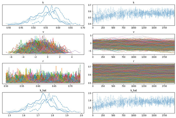
Here is the traceplot of the model with invlogit(r)

You could find out that r_ have high probability on 0.75, and less on 0.25.

Words are powerless to express my gratitude.

1 Like

Are those values unlikely? Maybe it makes more sense to plot them across trial number to see how they change over time. Having them overlaid on top of each other makes it difficult to gauge the uncertainity / bias