Deterministic variable gets split in summary

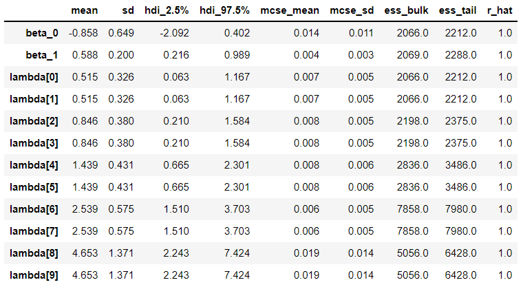
Why does my Deterministic variable (lambda in this case) get split into multiple components in the summary? I see that it’s the same number as the length of my data, but I don’t know where the connection is.

Here is the code:

import arviz as az
import matplotlib.pyplot as plt
import numpy as np
import pymc3 as pm

X = np.array((0., 0., 1., 1., 2., 2., 3., 3., 4., 4.))
y = np.array((0., 0., 1., 1., 2., 2., 3., 3., 4., 4.))

with pm.Model() as m:
    # priors
    beta_0 = pm.Normal("beta_0", mu=0, sigma=1000)
    beta_1 = pm.Normal("beta_1", mu=0, sigma=1000)
    
    lambda_ = pm.Deterministic("lambda", pm.math.exp(beta_0 + beta_1 * X))

    # likelihood
    y_pred = pm.Poisson("y_pred", lambda_, observed=y)

    # start sampling
    trace = pm.sample(
        3000,  # samples
        chains=4,
        tune=1000,
        init="jitter+adapt_diag",
        random_seed=1,
        return_inferencedata=True,
    )
    
az.summary(trace, hdi_prob=0.95)

Here is the summary output:

1 Like

Welcome!

In your data, X is a vector (1D matrix), so pm.math.exp(beta_0 + beta_1 * X) will be a vector as will lambda. Were you expecting something different? If so, what?

I you would like the mean of lambda over the whole vector (instead of only along the chain and draw dimensions) you should take a look at Working with InferenceData — ArviZ dev documentation. The summary function doesn’t do any extra aggregation because several quantities wouldn’t make much sense. But as you will see in the guide you can compute any of these aggregations manually with xarray and (with ArviZ development version, still unreleased right now) you can also plot aggregating any combination of dimensions with combine_dims.

Thanks cluhmann! I was expecting lambda to just be on its own line, without having been split into components.

Here is a example that I ran myself and got the results I was expecting (sigma and phi aren’t split into components):

baseline = np.array((5.9, 7.6, 12.8, 16.5, 6.1, 14.4, 6.6, 5.4, 9.6, 11.6, 
                     11.1, 15.6, 9.6, 15.2, 21.0, 5.9, 10.0, 12.2, 20.2, 
                     6.2))
after = np.array((5.2, 12.2, 4.6, 4.0, 0.4, 3.8, 1.2, 3.1, 3.5, 4.9, 11.1,
                  8.4, 5.8, 5, 6.4, 0.0, 2.7, 5.1, 4.8, 4.2))

with pm.Model() as m:
    # priors
    mu = pm.Normal("mu", mu=0, sigma=316)
    prec = pm.Gamma("prec", alpha=0.001, beta=0.001)
    sigma = pm.Deterministic("sigma", 1 / pm.math.sqrt(prec))

    ph1 = pm.Deterministic("ph1", switch(mu >= 0, 1, 0))

    diff = pm.Normal("diff", mu=mu, sigma=sigma, observed=baseline - after)

    # start sampling
    trace = pm.sample(
        10000,
        chains=4,
        tune=500,
        cores=4,
        init="jitter+adapt_diag",
        random_seed=1,
        return_inferencedata=True,
    )
    
az.summary(trace, hdi_prob=0.95)

OK I see now what the difference is between my code and the example in my reply.

The data is feeding directing into the Deterministic variable in my code, whereas it doesn’t in the example.

If I want to combine those components of lambda, I can do so with OriolAbril’s suggestions.

Thank you!

1 Like