Suppose I have data like:
n = 40
mu1 = 100
mu2 = 200
mu_array = np.ones(n) * mu1
mu_array[n//2:] = mu2

xs = np.array(range(n))
np.random.seed(1234)
ys = np.random.poisson(mu_array, size=n)

fig, ax = plt.subplots()
ax.scatter(xs, ys)
ax.set_xlabel("x")
ax.set_ylabel("y")
ax.set_ybound(0, None)
plt.show()
The idea is that there is some underlying latent parameter \mu_t, which is constant most of the time. But sometimes, it jumps to a totally different value in some wide range. We could model it by supposing that at each discrete time t, we roll a biased coin S_t \sim \mathrm{Bernoulli}(p), where p is small, say 0.01. When S_t = 0, \mu_t = \mu_{t-1}. When S_t = 1, \mu_t \sim \mathrm{SomeDistribution}(...), which could be something fairly flat like a Uniform, or a Gamma with a large variance. For simplicity I’ll go with a Uniform.
We don’t observe \mu_t directly, instead at each time step we observe a single count observation from a \mathrm{Poisson}(\mu_t).
Note: this isn’t about trying to estimate the location of a single switchpoint, as in the coal mining example in the docs. The example data has one jump, but in general there could be arbitrarily many. For instance, it could look like:
np.random.seed(222222)

mus = []
counts = []
n = 200
for _ in range(n):
    if np.random.random() < 0.01:
        mu = np.random.uniform(0, 500)
    else:
        mu = mus[-1] if mus else 100

    count = np.random.poisson(mu)
    counts.append(count)
    mus.append(mu)

fig, ax = plt.subplots()
ax.scatter(np.array(range(n)), counts)
plt.show()
But I want to at least get it to work on the simple dataset first.
First, can this kind of model even be fit in pymc? I think there would be gradient difficulties due to branching on the result of the Bernoulli cointoss, and I don’t know if that’s fatal or can be worked around. Second, if it is doable, how do I do it properly? Here is a naive attempt, that I didn’t really expect to work:
with Model() as model:
    mus = []
    for n, y in enumerate(ys):
        if len(mus) == 0:
            prior_mu = pm.Uniform(f"mu_{n}", lower=0, upper=500)
        else:
            switch = pm.Bernoulli(f"switch_{n}", p=0.01)
            prior_mu = pm.Deterministic(
                f"mu_{n}",
                pm.math.switch(
                    switch > 0,
                    pm.Uniform(f"unif_{n}", lower=0, upper=500),
                    mus[-1]
                )
            )

        new_mu = pm.Poisson(f"y_{n}", mu=prior_mu, observed=y)
        mus.append(new_mu)

    idata = sample(5000, target_accept=0.98)
Multiprocess sampling (4 chains in 4 jobs)
CompoundStep
>NUTS: [mu_0, unif_1, unif_2, unif_3, unif_4, unif_5, unif_6, unif_7, unif_8, unif_9, unif_10, unif_11, unif_12, unif_13, unif_14, unif_15, unif_16, unif_17, unif_18, unif_19, unif_20, unif_21, unif_22, unif_23, unif_24, unif_25, unif_26, unif_27, unif_28, unif_29, unif_30, unif_31, unif_32, unif_33, unif_34, unif_35, unif_36, unif_37, unif_38, unif_39]
>BinaryGibbsMetropolis: [switch_1, switch_2, switch_3, switch_4, switch_5, switch_6, switch_7, switch_8, switch_9, switch_10, switch_11, switch_12, switch_13, switch_14, switch_15, switch_16, switch_17, switch_18, switch_19, switch_20, switch_21, switch_22, switch_23, switch_24, switch_25, switch_26, switch_27, switch_28, switch_29, switch_30, switch_31, switch_32, switch_33, switch_34, switch_35, switch_36, switch_37, switch_38, switch_39]

Sampling 4 chains, 0 divergences ━━━━━━━━━━━━━━━━━━━━━━━━━━━━━━━━━━━━━━━━ 100% 0:00:00 / 0:02:09

Sampling 4 chains for 1_000 tune and 5_000 draw iterations (4_000 + 20_000 draws total) took 130 seconds.
/nix/store/0p0m0595a9q7m19x35xvydv5h9irg9gi-python3-3.11.9-env/lib/python3.11/site-packages/arviz/stats/diagnostics.py:592: RuntimeWarning: invalid value encountered in scalar divide
  (between_chain_variance / within_chain_variance + num_samples - 1) / (num_samples)
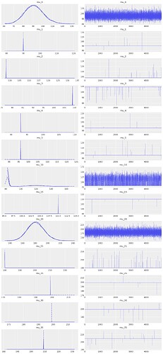
As I sort of expected, this is an abject disaster:
az.plot_trace(idata, var_names=["mu_0",
                                "mu_1", "mu_2", "mu_3", "mu_4", "mu_5",
                                "mu_10", "mu_15", "mu_20", "mu_21", "mu_25", "mu_30", "mu_35"
                               ])
Some of the traces look reasonable, others are almost Dirac-delta singularities, others are bimodal and spread across the parameter range. Not good!
I don’t understand pymc well enough to know if this is just because I’m implementing the model wrong, or if it’s intractable in any case. Can anyone shed some light? I’m also open to other ways of modelling the data … anything that will behave like “constant most of the time, with occasional large jumps”.


