Hello,
I hope this isn’t a totally novice question - I’ve done some digging around on these forums and elsewhere to try and see if I’m implementing my problem correctly but I thought I’d ask it here just in case.
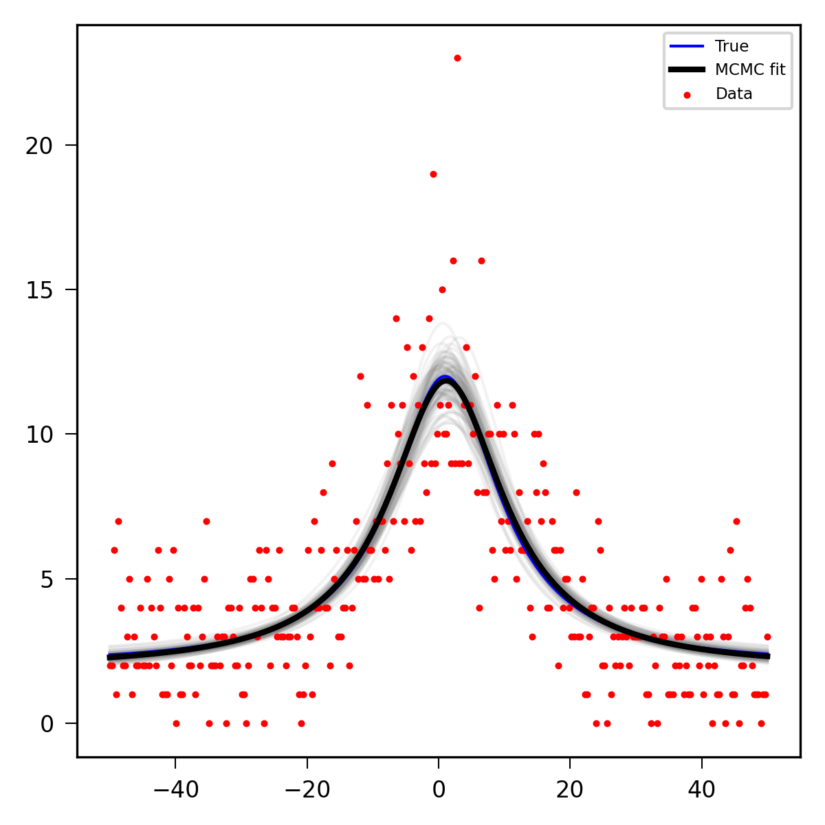
I’m trying to fi ta function (here, a Lorentzian peak + flat background) to data that is generated by Poisson sampling (e.g. by counts hitting a detector and populating a histogram).
Below I have (hopefully) implemented a Poisson likelihood for the data (obs) and some Normal / HalfNormal priors for the fitting variables. I got a good match with the interfered parameters + fit and the true distribution. But my questions are:
-
Is this the correct way to handle Poisson distributed data? Is it even appropriate to call it ‘Poisson distributed’, or is the distribution function actually my fit equation ‘mu’ (Lorentzian + background)?
-
Do I instead need to define a variable that accounts for Poisson noise? If so, then what sort of distribution do I use for the ‘obs’ variable?
Thanks very much for any feedback you may have (directly relevant to the problem or any advice at all on how to better implement this)!
import arviz as az
import matplotlib.pyplot as plt
import numpy as np
import pymc3 as pm
np.random.seed(12345)

# Parameters for data and function
c0    = 2 # Background constant
amp   = 100 # Peak amplitude
x0    = 1 # Offset
gamma = 20 # FWHM

x = np.linspace(-50, 50, 300)
y_true = c0+amp*(1/2)*gamma/((x-x0)**2+(1/2*gamma)**2)
y = np.random.poisson(y_true, size=len(y_true))

fig1 = plt.figure(1, dpi=150, figsize=(4, 4))
plt.scatter(x, y, color='r', s=2, label="Data")
plt.plot(x, y_true, color='b', lw=1, label="True")
plt.legend()
plt.tight_layout()

var_names = ["c0", "amp", "x0", "gamma"]

if __name__ == "__main__":
    with pm.Model() as model:
        c0    = pm.HalfNormal('c0', sigma=5, testval=1)
        amp   = pm.Normal('amp', mu=100, sigma=20, testval=100)
        x0    = pm.Normal('x0', mu=1, sigma=10, testval=1)
        gamma = pm.Normal('gamma', mu=20, sigma=10, testval=20)
        mu    = pm.Deterministic('mu', c0+amp*(1/2)*gamma/((x-x0)**2+(1/2*gamma)** 2))
        obs   = pm.Poisson('obs', mu=mu, observed=y)

    with model:
        trace = pm.sample(3000, chains=2, cores=1)
        trace = trace[1000:]

    with model:
        az.plot_trace(trace, var_names=var_names, figsize=(8, 6))

    with model:
        ppc = pm.sample_posterior_predictive(trace, var_names=var_names, random_seed=42)
        ppc_fit = pm.sample_posterior_predictive(trace, var_names=['mu'], samples=100, random_seed=42)

    y_MCMC = trace.mu.mean(0)

    plt.figure(1)
    plt.plot(x, y_MCMC, color='k', lw=2, label='MCMC fit') # plot trace mean for mu
    [plt.plot(x, y, color=[0.5, 0.5, 0.5], alpha=0.1, zorder=0) for y in ppc_fit['mu'][0:100]] # plot 100 posterior samples of mu
    plt.legend()