It’s probably rather simple, but I don’t understand why I cannot evaluate the conditional covariance function. I’ve adapted this example of a homoskedastic GP as a minimal working example.
1. Creating the data
import numpy as np
import pymc as pm


def signal(x):
    return x / 2 + 2 * np.sin(2 * np.pi * x)


def noise(y):
    return np.exp(y) / 10


SEED = 2020
rng = np.random.default_rng(SEED)

n_data_points = 4
n_samples_per_point = 8
X = np.linspace(0.1, 1, n_data_points)[:, None]
X = np.vstack([X, X + 2])
X_ = X.flatten()
y = signal(X_)
σ_fun = noise(y)

y_err = rng.lognormal(np.log(σ_fun), 0.1)
y_obs = rng.normal(y, y_err, size=(n_samples_per_point, len(y)))
y_obs_ = y_obs.T.flatten()
X_obs = np.tile(X.T, (n_samples_per_point, 1)).T.reshape(-1, 1)
X_obs_ = X_obs.flatten()
idx = np.tile(
    np.array([i for i, _ in enumerate(X_)]), (n_samples_per_point, 1)
).T.flatten()

Xnew = np.linspace(-0.15, 3.25, 100)[:, None]
Xnew_ = Xnew.flatten()
ynew = signal(Xnew)
2. Fit the model
coords = {"x": X_, "sample": np.arange(X_obs_.size)}

with pm.Model(coords=coords) as model_hm:
    _idx = pm.ConstantData("idx", idx, dims="sample")
    _X = pm.ConstantData("X", X, dims=("x", "feature"))

    η = pm.Exponential("η", lam=1)
    ell_params = pm.find_constrained_prior(
        pm.InverseGamma, lower=0.1, upper=3.0, init_guess={"mu": 1.5, "sigma": 0.5}
    )
    ℓ = pm.InverseGamma("ℓ", **ell_params)
    cov = η**2 * pm.gp.cov.ExpQuad(input_dim=1, ls=ℓ) + pm.gp.cov.WhiteNoise(1e-6)
    σ = pm.Exponential("σ", lam=1)

    gp_hm = pm.gp.Latent(cov_func=cov)
    f = gp_hm.prior("f", X=_X)
    ml_hm = pm.Normal("ml_hm", mu=f[_idx], sigma=σ, observed=y_obs_, dims="sample")

    trace_hm = pm.sample(
        500,
        tune=1000,
        chains=1,
        return_inferencedata=True,
        random_seed=SEED,
        nuts_sampler="numpyro",
    )
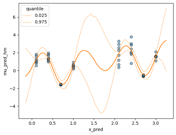
3. Make predictions
with model_hm:
    model_hm.add_coords({"x_pred": Xnew_})
    mu_pred_hm = gp_hm.conditional("mu_pred_hm", Xnew=Xnew, dims="x_pred")
    samples_hm = pm.sample_posterior_predictive(
        trace_hm, var_names=["mu_pred_hm"], random_seed=42
    )
4. Sampling the posterior covariance function
Until here, everything looks fine to me. Now, I’d like to sample the posterior covariance function for my observed data.
with model_hm:
    jitter = 1e-6
    givens = gp_hm._get_given_vals(None)
    mu2, cov2 = gp_hm._build_conditional(_X, *givens, jitter)
And this is where I’m stuck.. How do I obtain the 8x8 covariance matrix for the observed data locations?