I want to try to model some data using a Poisson Mixture Model with 2 components. As I am new to PyMC3, I used the links here: GMM tutorial and here: Mixture Models API to try to do this. My code is here:
Doing proper inference for mixture model is not easy - if you do a search on the discourse there are a few pointer to better parameterize your model (e.g., Properly sampling mixture models)
First, you need to make sure the inference is done correctly. Plot the trace and check that: there is no divergence, no rhat and effective sample size warning, and in general the trace looks fine.
@cynthiaw2004 , I’ve tried running that model a few times on separate days. Using your parameters, the model converged successfully after about 6 trials. I’m not sure why it takes so many trials to converge, but I never got it on the first time. When the model didn’t converge (Rhat > 1), it is quite obvious in the visualization below:
But when it converged, you can see the visual alignment:
Like @Junpenglao suggested, it would be best if you separate the model into groups such as follows:
with pm.Model() as model:
    lam1 = pm.Exponential('lam1', lam=1)
    lam2 = pm.Exponential('lam2', lam=1)
    pois1 = pm.Poisson.dist(mu=lam1)
    pois2 = pm.Poisson.dist(mu=lam2)
    w = pm.Dirichlet('w', a=np.array([1, 1]))
    like = pm.Mixture('like', w=w, comp_dists=[pois1, pois2], observed=data)
with model:
    trace = pm.sample(5000, n_init=10000, tune=10000, random_seed=SEED)[1000:]
Then try: pm.summary(trace)
or: pm.forestplot(trace)
to confirm that the model converged.
I think we can help the model converge on the first trial by setting testval=something within pm.Exponential('lam1', lam=1), but I’m not sure what that should be equal to in this case.
Restricting the order of the location parameter (lam in this case) usually prevents label switching and helps convergence - although your model still can be unidentifiable if you dont have enough data or the latent mixture location is too close. For more detail see Mike Betancourt’s case study (I have a PyMC3 port for this).
In this case, applying the similar parameter constrains:
import pymc3.distributions.transforms as tr
chain_tran = tr.Chain([tr.log, tr.ordered])

with pm.Model() as model:
    lam = pm.Exponential('lam', lam=1,
                         shape=2,
                         transform=chain_tran,
                         testval=np.asarray([1., 1.5]))
    pois = pm.Poisson.dist(mu=lam)
    w = pm.Dirichlet('w', a=np.array([1, 1]))
    like = pm.Mixture('like', w=w, comp_dists=pois, observed=data)
Thanks for the suggestions. I did get a “The estimated number of effective samples is smaller than 200 for some parameters” so I upped the draws parameter for the sample function to make that go away. I also used traceplot (attached)
and checked the rhats using summary(trace), but the rhats are not looking too hot…
As for your suggestion on using tr.Chain, I am getting an attribute error: AttributeError: module ‘pymc3.distributions.transforms’ has no attribute ‘Chain’
I am using the git version of pymc3 (not the pip version) so any ideas what is going on there?
You say you got it to converge after 6 trials. I apologize for the beginner question, but is that a parameter in the sample function? If so, which? sample api
Or that you just ran sample 6 times? And on the 6th time it finally converged?
@cynthiaw2004 I meant that I ran it 6 or 7 times when it finally converged. Your summary trace results appear to be pretty good, suggesting a nice convergence.
If you’d like to visually compare the observed data with the posterior trace results, this should work:
N = 1000                              # this is the size of your observed data number

W = np.array([0.18, 0.81])            # these are the means of the w's in your summary(trace)

Lam = np.array([281.91, 1032.00])     # these are the means of the Lam's

# Simulate a Poisson distribution from the posterior parameters
component = np.random.choice(Lam.size, size=N, p=W)
x = np.random.poisson(Lam[component], size=N)

fig, ax = plt.subplots(figsize=(8, 6))

# Histogram of the original, observed data
ax.hist(observed_data, bins=20, normed=True, lw=0, alpha=.8, label='Observed data')

# Histogram of the simulated posterior parameters from above
ax.hist(x, bins=20, normed=True, lw=0, alpha=0.4, color='gray', label='Posterior traced distribution')

sns.kdeplot(x, label='Posterior traced KDE')
sns.kdeplot(observed_data, label='Observed data KDE')
plt.legend()
plt.show()
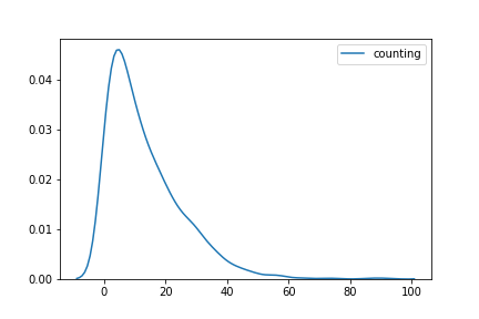
Thanks. However, the graph still looks wrong…attached below. Also, sorry if I made it ambiguous but I am using the data in the text file below which is not exactly the data used in the tutorial above.
Thanks, I git pulled. Although now I get the error: ValueError: Mass matrix contains zeros on the diagonal.
The derivative of RV w_stickbreaking__.ravel()[0] is zero.
I also tried this data out with the Chapter 1 code involving switchpoints in the Probabilistic Programming and Bayesian Methods for Hackers book. This gave me this figure which I think is decent. But I would still really like it if I could somehow use mixture models. In addition, there is the possibility that multiple taus exist, and knowing how many beforehand without looking ahead of time at the graph is not obvious to me.
@cynthiaw2004 you shouldn’t be using mixture model for this. If you’re interesting in seeing where the count of x had a sudden change, as the hours pass by, switchpoint is a good option. Mixture models is not what you’re looking for.
Do you have any suggestions on how to deal with the possibility of multiple taus? Let’s say I could not look at the graph beforehand. Looking at the graph above is sort of cheating because I already know there are two pieces separated by one tau. Can I account for any number of taus?
You are asking about estimating the number of clusters within a data set. That is complicated; there is no simple way to do that. But I would continue reading material on the usage of pymc3 and bayesian statistics before you worry too much about this advanced material. Try and get through more chapters of the book and things will clear up a bit.