Is it legitimate to perform a Prior Predictive Check in this way?

I would like to have from you an approval or a disapproval for the following method, by which I thought to carry out a prior predictive check, without going through the functions of the ArviZ module.

Note that I’m not trying to find out if the method is really practical, but if it makes sense to do things like that and if it doesn’t contain errors in reasoning.

So, I start from a beta-binomial model (traditional coin-flip model) where the parameter theta is modeled by the prior Beta, say Beta(0.5, 0.5).

I programmed a series of n=73 Bernoulli experiments and my result shows x_{obs}=46 successes. I wonder how could I quantify the fact that my prior is adequate or not.

This article by Coon et al. HERE gives (in its table 2) several “discrepancy functions and pivotal quantities useful for Bayesian model checking” (as quoted), and it seemed useful to me to use the first function (referenced \chi^2), modifying it with a logarithm np.log() so as to reduce excessive variations.

Concretely, for a given \theta parameter, taking into account that the expected number of successes x is n\theta, I calculate the discrepancy value T between a given x (either predicted by sampling or observed) and its expectation, by the formula:
T(x,\theta)=np.log(\frac{(x-n\theta)^2}{n\theta})

My procedure is:

  • to carry out a number N of random draws of the \theta parameter from the prior (say, \theta_i),

  • then, for each \theta_i obtained, to get a number x_i of predicted successes by random draw from the corresponding sampling distribution (i.e. the binomial law Binom(n=73, \theta= \theta_i))

  • and then to apply the discrepancy function T to the (random) value x_i \rightarrow T(x_i, \theta_i) and to the (fixed) value x_{obs} \rightarrow T(x_{obs}, \theta_i) .

This gives me N couples (T(x_i, \theta_i), T(x_{obs}, \theta_i)), for each of which I express the Boolean result (T(x_{obs}, \theta_i) > T(x_i, \theta_i)) as 0 (False) or 1 (True).

Now, the proportion of 1 should give me an approximate value of the probability p that the observed data lie beyond the predicted data.

And, as far as I understand from the usual rules, the model is fit if p\sim0.5 and misfit if p\sim0 or p\sim1

The program I used to do so is:

fixing the number of Bernoulli trials

n = 73

fixing the number of observed successes during the trial

x_obs = 46

fixing the parameters of the beta prior

alpha, beta = 0.5, 0.5

fixing the number of draws

draws = 20000

sampling parameter values (\theta) from the prior

thetas = np.random.beta(alpha, beta, size = draws).tolist()

sampling successes x from the likelihood (with the given sampled \theta)

predicted = [np.random.binomial(n, theta, size = 1)[0] for theta in thetas]

expected values from the given likelihood (binomial distribution)

expected = [theta*n for theta in thetas]

assess discrepancies T (through \log(chi^2) computation) for predicted x

T_predicted = [np.log((x - y)**2 / y) for (x, y) in zip(predicted, expected)]

assess discrepancies T (through \log(chi^2) computation) for observed x_{obs}

T_observed = [np.log((x_obs - y)**2 / y) for y in expected]

check when T_observed > T_predicted

checks = [x > y for (x, y) in zip(T_observed, T_predicted)]

other statistics

mean_T_predicted = sum(T_predicted)/len(T_predicted)
mean_T_observed = sum(T_observed)/len(T_observed)

prob = sum(checks)/len(checks)

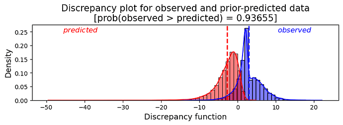
Plotting the N values of the calculated discrepancy function gives me:

I think the plot shows a characteristic pattern of a misfit model. The p-value calculated, which of course varies each time the program is restarted, was 0.93655 in my own run, which confirms, if this procedure is indeed valid, that the model is inadequate, leading to the conclusion that I should change my prior.

I’m sorry it took a bit long to explain… Do you agree with all this ? Do you have any comments (deeply appreciated)?
Hi Andre!

I’m having trouble resolving the conceptual motivation for this. Ultimately, you want your prior distribution to represent either the information that you have available regarding the unknown parameters before observing the data, or to represent the population of plausible values of those parameters. So, a prior is only inappropriate if it fails to satisfy either of these criteria. From a practical standpoint, informative priors can help to constrain the parameter space to make them easier to fit.

So in your case, a Beta(0.5, 0.5) prior is only inappropriate if it does not capture the prior information for your problem. If I swap in, say, a Beta(2, 2) prior it makes no real difference to the posterior estimate of p, so your problem is pretty insensitive to a pretty wide range of weakly-informative priors. If instead I knew that in 5 previous experiments there were 3 successes, then a Beta(3, 2) prior would be a good choice. Even still, it would not change the posterior inference meaningfully if you used your prior instead.

Paul Conn’s article focuses primarily on posterior checks, which are very important. There is a small section on prior checks, from which the takeaway message is that they aren’t used much in practice. I only use them to make sure that the prior predictive samples aren’t orders of magnitude away from the plausible range of parameter values that I expect.

3 Likes

Hi Chris,

Thank you for your answer. I understand your misunderstanding! I myself am not very sure of what I am doing… Let’s say that I am looking for possibilities to do, to see what happens, hoping to better understand notions that I do not yet master…

Regarding these famous prior predictive checks, I can read this, for example:

  • In “Bayesian Analysis Reporting Guidelines” (HERE):

“Prior predictive check. especially when using informed priors but even with broad priors, it is valuable to report a prior predictive check to demonstrate that the prior really generates simulated data consistent with the assumed prior knowledge.”

“A prior predictive check displays simulated data that are generated from parameter values in the prior distribution. The simulated data from the mathematically specified prior should show trends that match the trends assumed by prior knowledge.”

  • In Prior predictive checks (Stan Software) (HERE):

“Prior predictive checks generate data according to the prior in order to assess whether a prior is appropriate”

Philosophically, I understand what that means, but, faced with a keyboard, a computer, a jupyter notebook and any model, I don’t see how to proceed concretely. So, I make myself the simplest possible model, for example Beta-binomial, I invent a prior and I say to myself: “good, and now, to carry out this prior predictive check that everyone is talking about, how do you do it?” So, I invent a way of doing things, such as the one described above, and I ask specialists if it makes sense or not… This is the explanation of the “conceptual motivation for this” you were asking for.

Having said this, I acknowledge that using Beta(\alpha, \beta) priors with varying \alpha and varying \beta, don’t make real difference (at least regarding the so-called “discrepancy function” I used), unless \alpha comes to \sim 50 and beta comes to \sim 25 … (where my so-called p-value comes to \sim 0.5).

Ultimately, to make it simpler and not get lost in the details, I might as well ask you the question abruptly: if you had to process a Beta-binomial model for which you are not sure of you prior, how would you proceed to carry out a prior predictive check to assess whether your prior is appropriate?

And thank you for your patience…

The prior is your “belief” about what the parameters might be like. Now people don’t usually have a good intuition about parameters, they have intuition about the data that is generated by the process they are studying (and parametrizing).

Prior predictive checks are a way to help users understand the implications of the parameter priors, by simulating data that respects those prior beliefs.

Once users have simulated data it’s easy (easier) to say: 1) this looks reasonable vs 2) these simulated values are completely insane! If 2) happens that means you must have specified “wrong” priors for your parameters (or the likelihood function is wrong).

The Stan documentation has an example for 2) in a model with a gamma prior and a poisson likelihood: 26.5 Example of prior predictive checks | Stan User’s Guide

Notice how the “unreasonableness” of the priors in that Stan example depends on the actual meaning of the data they are modelling. Maybe part of the conceptual challenge you’re facing is that you are not thinking about a realistic model with specific data. Once you have that it might be more obvious how a prior predictive check helps because you will have real intuitions about 1) vs 2).

Hi Ricardo,

Sorry for not having answered sooner; I was away for a few days…

You say: “Once you have [data] that it might be…”; but I have data: as I previously said, my result shows x_{obs}=46 successes.

So, let me modify my previous code for a simpler one:

import seaborn as sns
import numpy as np
import matplotlib.pyplot as plt
from scipy.stats import beta, binom

prior_alpha = 0.5
prior_beta = 0.5
n = 73
x_obs = 46

Generate samples from the prior distribution

prior_samples = beta.rvs(prior_alpha, prior_beta, size = 20000)

Simulate the prior predictive distribution

prior_predictive_samples = [binom.rvs(n, p) for p in prior_samples]

Calculate the proportion of prior predictive samples equal to or more extreme than the observed data

count_extreme = sum(sample >= x_obs for sample in prior_predictive_samples)
proportion_extreme = count_extreme / len(prior_predictive_samples)

Plot the histogram of the prior predictive samples

fig, ax = plt.subplots(1, 1, figsize = (8,4), tight_layout=True)

sns.histplot(data = None, x = prior_predictive_samples, binwidth = 1, discrete = True, shrink = 1.0,
stat = “density”, element = “bars”, color = “blue”, kde = True)

ax.axvline(x_obs, color = “red”, ls = ‘–’, lw = 2, label = “Observed Data”)

ax.set_title(f"Prior Predictive Distribution and observed data" + “\n”
+ r"prior = \, \theta \sim Beta" + f"({prior_alpha}, {prior_beta})" + " - | - "
+ r"x_{observed} = 46" + “\n”
+ f"[proportion(prior predictive samples >= {x_obs}) = {proportion_extreme}]“,
fontsize = ‘15’)
ax.set_xlabel(r"Number x of successes” , fontsize = ‘13’)
ax.set_ylabel(“Density”, fontsize = ‘13’)

plt.legend()
plt.show()

Can I now call this a Prior Predictive Check? And what kind of conclusions could I draw from the plot produced? Or is it still inaccurate / inappropriate / illogical to perform a Prior Predictive Check in this way for a simple beta-binomial model?

Any advice appreciated…

You have 46 successes but what do those mean in the real world?

It’s different if I am talking about flipping a coin a couple of times or counting the number of correct answers in a highly demanding quizz. When you have a real wold problem your data will have a meaning and you will have grounded expectations about what that data may look like. That’s when prior predictive checks are useful.

If you are simulating data from a black-box random number generator then prior predictive checks may not be very useful. Your results show your prior is compatible with anything between 0 or 70? Is this reasonable or not? In a real word setting you would have an answer for this.

To answer your more direct question. There is no way I know of that a prior predictive check can be invalid, it’s just a simulation. The worse that can happen is that they are not useful for your goal and you wasted some CPU cycles.

Taking a step back, I am not sure what you are asking. Prior predictive checks are just one tool in the model building arsenal. I’ve been trying to hint at the most typical use case of this tool, but there is no right or wrong answer when you are using a tool. It may just be more or less fit for the job compared to other tools.

Ok, I understand better that it’s not the procedure used that was actually meaningless (with an unsolvable question: is it valid, or is it invalid? ); in fact, it was the question itself that prompted the procedure that was meaningless…

Because yes, it’s true, the problem posed does not come from the real world; it’s actually totally artificial, and that’s what must confuse people used to resolving Bayesian inferences from real situations.

It was designed as a practice for me to answer questions such as "what is a prior predictive check? how does it work? how is it coded (in Python)? what can I say of the results I get? etc…

Learning questions, if I may say so.

Anyway, thank you for taking the time to make things clearer.

Thanks for posing the questions, it’s very helpful for me to try and think these things over and from a different perspective.

I don’t consider the matter solved, I just tried to convey my best understanding up to date. I will be happy to follow this thread and see if other people have different suggestions on how to answer your questions.

As a sidenote, 99% of the work I do is with simulations and I think that’s a great way to learn. It’s just that sometimes it helps to pretend these simulated numbers live outside of the machine :slight_smile:

Happy learning!