Hello,
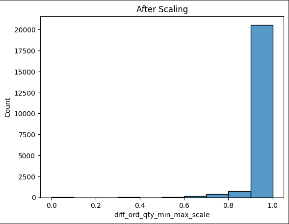
Has anyone had an issue using a truncated normal distribution for the likelihood? I’m trying to do a very simple model estimating my target variable which has been scaled between [0,1]. The model using a normal distribution for the likelihood is below.
coords = {'cann':[1,0]}
with pm.Model(coords = coords) as cannibal_model:
cannibal = pm.Data('cannibal', cann_idx, mutable = True)
obs = pm.Data('obs', obs_array, mutable = True)
# beta = pm.Normal('beta', mu=0, sigma = .1)
alpha = pm.Normal('alpha', mu=0, sigma = .05, dims = ['cann'])
mu = alpha[cannibal]
sigma = pm.HalfCauchy('sigma', beta=0.1)
eaches = pm.Normal('predicted_eaches',
mu=mu,
sigma=sigma,
# lower = 0,
# upper = 1,
observed=obs)
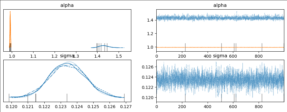
idata = pm.sampling_jax.sample_numpyro_nuts(draws = 1000, tune=2000, target_accept = .95)
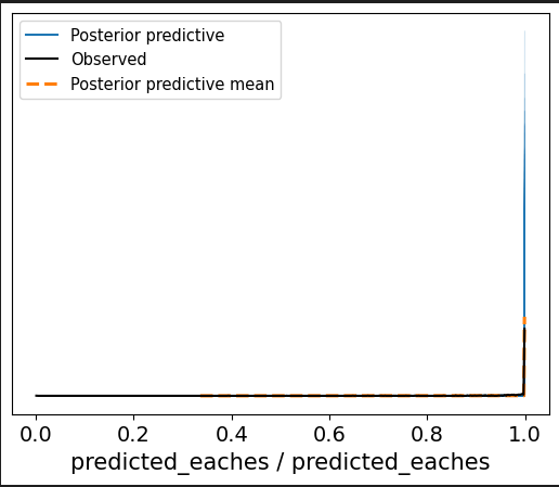
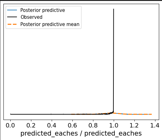
This gives me a great trace plot but my ppc is estimating above 1.
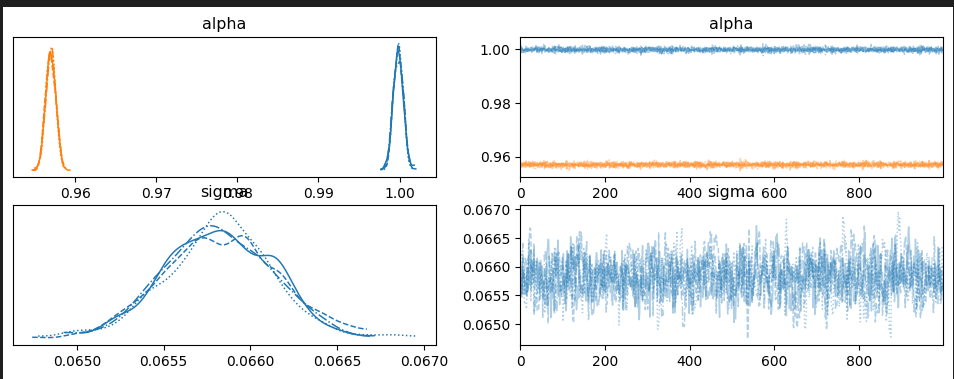
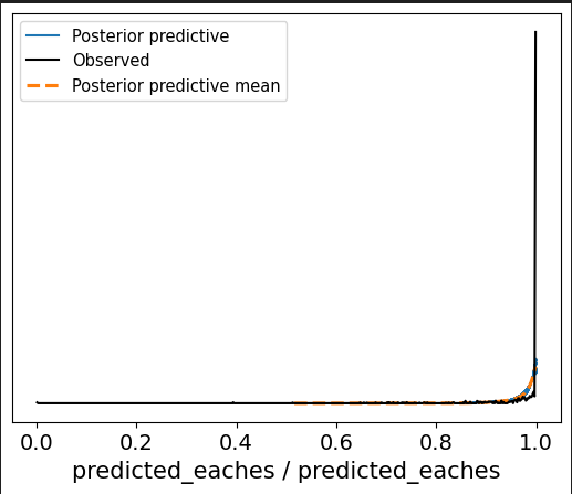
When I run the following using a truncated normal for the likelihood, as below, the trace looks off but the ppc looks…better.
coords = {'cann':cann}
with pm.Model(coords = coords) as cannibal_model:
    cannibal = pm.Data('cannibal', cann_idx, mutable = True)
    obs = pm.Data('obs', obs_array, mutable = True)

   #  beta = pm.Normal('beta', mu=0, sigma = .1)
    alpha = pm.Normal('alpha', mu=0, sigma = .05, dims = ['cann'])

    mu = alpha[cannibal]
    sigma = pm.HalfCauchy('sigma', beta=0.1)

    eaches = pm.TruncatedNormal('predicted_eaches',
                           mu=mu,
                           sigma=sigma,
                        #    lower = 0,
                           upper = 1,
                           observed=obs)

    idata = pm.sampling_jax.sample_numpyro_nuts(draws = 1000, tune=2000, target_accept = .95)
Is this a parameters issue or is this indicative of a truncated normal distro?