Lagged Time Series with delayed and gradual effects

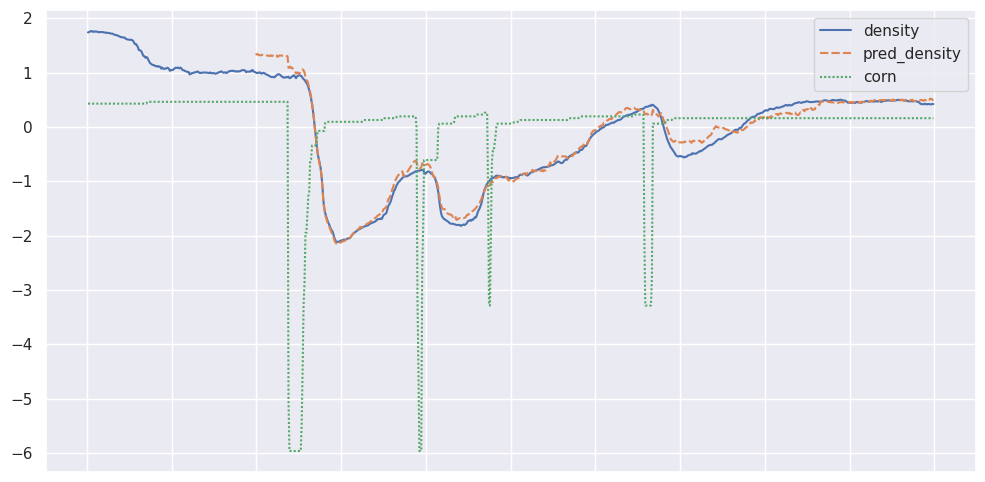
I am trying to model an industrial process in which corn and water are mixed together and cooked in 2 large mixing tanks before flowing out to the next step of the process. There is a density meter on the outflow. The system runs continuously so there is almost always water and corn coming in and the cooked product coming out. Here is a graph of the standardized corn, water, and density:

The x axis is in minutes.

I want to build a model that predicts the density given the corn and water flow rates. More corn and less water makes the density go up but because of mixing there is a time delay and the effect of turning off the grind for a few minutes doesn’t produce an immediate and corresponding drop in the density. The density decreases gradually in response to the corn flow stopping then comes back up gradually after the water flow is reduced. I also have other variables I would like to include such as the temperatures and levels of both tanks and the flow rate out of the entire system which might affect the lag time.

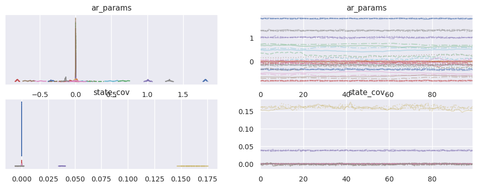
What kind of model can I use for this? I have been experimenting with BayesianVARMAX by trying the notebook here but it takes multiple hours to sample a small subset of the data. I also don’t see a place where I can put in exogenous vs endogenous variables.

Should I use gaussian processes? gaussian random walks? Some other kind of model?

Can you post an example of a VARMAX model you’ve tried so far? “It’s slow” is hard to diagnose. I can say that indeed, in the default C backend, statespace models can be slow. It is recommended to use JAX. Priors and identification are also exceedingly important to speed in VARMA models, especially at higher orders or if you’re MA components (I don’t recommend you use MA components).

As for exogenous variables, I just merged a PR that adds this functionality – you can see examples in the tests here. I haven’t updated the VARMAX notebooks to show how it works yet.

Moving beyond the statespace model, you can do VAR models “by hand” in PyMC quite easily by just making lagged feature matrices and doing linear regression. The downside of this approach is that you don’t get forecasting/filtering/irf “for free”, which is what the statespace machinery buys you. Examples here and here.

ss_mod = pmss.BayesianVARMAX(order=(2, 0),
                             endog_names = data.columns,
                             stationary_initialization=False,
                             measurement_error=False)


with pm.Model(coords=ss_mod.coords) as var_model:
    
    # For x0, I choose something very close to 0, since that's the steady-state of the stationary model
    x0 = pm.Normal('x0', sigma=0.1, dims=['state'])
    
    # For P0, we find a Gamma prior with 95% of the mass between 0.5 and 2, which I took by looking at the data
    P0_diag = pm.Gamma('P0_diag', **pm.find_constrained_prior(pm.Gamma, 
                                                  lower=0.5, 
                                                  upper=2.0, 
                                                  init_guess={'alpha':2, 'beta':1}),
                      dims=['state'])
    
    P0 = pm.Deterministic('P0', pt.diag(P0_diag), dims=['state', 'state_aux'])
    ar_params = pm.Normal('ar_params', dims=['observed_state', 'lag_ar', 'observed_state_aux'])
    
    # Let's also upgrade the shock covariance to be dense, rather than diagonal
    state_chol, *_ = pm.LKJCholeskyCov('state_chol', n=data.shape[1], eta=1, sd_dist=pm.Exponential.dist(1))
    state_cov = pm.Deterministic('state_cov', state_chol @ state_chol.T, dims=['shock', 'shock_aux'])
    
    ss_mod.build_statespace_graph(data, mode='JAX')
    prior = pm.sample_prior_predictive()
    idata = pm.sample(draws=100, tune=100, nuts_sampler='numpyro')

az.plot_trace(idata, var_names=['ar_params', 'state_cov'])

That’s the VARMAX model I ran. I copied your notebook exactly and swapped in my data :slight_smile:

It took ~4 hours to run a mere 200 draws. I have read many discussions on this discourse about sampling speed and have done all the backend optimizations. I even bought hardware specifically for running pymc. I have greatly reduced sampling times for other models so in this case it is likely an issue with the way I have specified the model.

The math and linear algebra involved in state space and multivariate time series is beyond my knowledge.

Here is my trace:

Well, 4 hours for 200 draws isn’t acceptable.

What are the dimensions of your data?

3 columns and 1500 rows

I got the new version of pymc_extras running and was able to try out the BayesianSARIMAX function.
I ended up downsampling to reduce the number of rows and taking the difference so I could use stationary initialization.

I also noticed you’re using the numpyro sampler, you might be a free speedup if you switch over to nutpie:

    idata = pm.sample(nuts_sampler='nutpie', nuts_sampler_kwargs={'backend':'jax', 'gradient_backend':'jax'})

If you check the other example notebooks (SARIMAX, ETS, structural), this is the setting we recommend. the VARMAX one is out of date and due for an update.

Otherwise, it would be good if we can do better on long time series. In the filtering literature it’s known that you can stop doing computation at some point, after which additional timesteps would be really cheap. There’s an issue about it here.

Were the timings on the SARIMAX run more reasonable? We also added exogenous variable support for VARMAX, so you can maybe try a system of water + density, with exogenous corn (or some other permutation).

1 Like

Also you shouldn’t have to difference your data to use the stationary initialization. In this context, “stationary” is a feature of the transition matrix, not the data. If you choose a Beta prior on your AR term, an AR(1, q) should always be stationary. For AR(2, q), use a Dirichlet for the two AR terms (the unit simplex is all stationary, though there are still some bad dynamics in there). For higher orders you have to get more creative.

I don’t think the plot you shared looks non-stationary anyway, for what it’s worth.

I have been trying a lot of different things. The nutpie sampler only takes ~15 minutes to run the 1000 draws + 1000 tuning samples on a 3000 row dataframe so that’s awesome.

Also I’ve been digging through the source code on github and the comments there are helpful.

Running a SARIMAX(0,0,1) model looks like this:

The predicted kind of follows the observed data. If I run a higher order model the prediction tightens up but the exogenous variables don’t have as much influence. I have been trying some VARMAX models with all three variables as endogenous as well.

The issue i see with the SARIMAX approach is that currently the exogenous data only enters contemporaneously (in your MA(1) case for example as y_t = \beta x_t + \theta \varepsilon_{t-1} + \varepsilon_t ) but looking at the graph, there’s definitely a lag between the shock to the corn and the change in density.

The only easy way to add in dynamic exogenous regressors at the moment is via VAR, which I recognize is a bit of a bummer. I guess people call it ARDL when you have something of the form y_t = \sum_{s=1}^S \rho_s y_{t-s} + \sum_{k=0}^K \beta_k x_{t-k}, which might be relevant to your case?

PS: Happy to hear the comments in the code are helpful! Feel free to open issues/PRs if anything seems wrong to you or isn’t clear.

PPS: It seems like the stationary initialization is doing something dumb in your case – you might get some lift by manually specifying x0 to be centered on the first datapoint. I’m thinking about making this the default and arguing that it’s “empirical bayes” – curious what you think.

I guess people call it ARDL when you have something of the form yt=∑Ss=1ρsyt−s+∑Kk=0βkxt−k, which might be relevant to your case?

Yes, I have been looking at ARDL and I think that is relevant in this case. I have tried implementing it with statsmodels and the results are pretty good.

This took 180 lags (data points are 2 mins apart) to get a good fit. I excluded the autoregressive order so I think this is just equivalent to making lagged columns for each feature and doing OLS? The output gave me a list of coefficients for water L1, water L2…water L180, corn L1, corn L2…

It seems like the stationary initialization is doing something dumb in your case – you might get some lift by manually specifying x0 to be centered on the first datapoint. I’m thinking about making this the default and arguing that it’s “empirical bayes” – curious what you think.

My first density datapoint is 1.745 so does that mean my model would look like this?

initial_x0 = data['density'].values[0]

with pm.Model(coords=sar_mod.coords) as sar_model:
    
    x0 = pm.Normal('x0', mu=initial_x0, sigma=1, dims=['state'])

or like this?

initial_x0 = data['density'].values[0]

with pm.Model(coords=sar_mod.coords) as sar_model:
    
    x0 = initial_x0

I have no problem doing ‘empirical bayes’ for this. My audience doesn’t care how I get there. They just care about prediction and interpretability. In this case they need to know how to bring the system back to steady state after a planned or unplanned shock.

Depends on the model you end using. x0 is a vector with one value per hidden state in the model, so you have to know what they all are. For an ARIMA you want to set the first element of the vector (that’s the “current level” state) with the data, then a bunch of zeros (warning, untested code):

data_t0 = data['density'].values.item(0)
with pm.Model(coords=sar_mod.coords) as sar_model:
    x0_vec = pt.zeros(sar_mod.k_endog)[0].set(data_t0)
    x0 = pm.Deterministic('x0', x0_vec, dims=['state'])

For the ARDL model, yes you are just doing a regression with a bunch of lagged features (actually all AR style models can be re-written this way). 180 lags is pretty crazy though.

I think there’s a way more simple physical processing going on in your data, where the rate of change of the density is shocked by corn variable, but the effect decays with an AR process, back to a steady state value. The only shock my proposed model doesn’t explain is the third one – there doesn’t seem to be any dip after that.

I think there’s a way more simple physical processing going on in your data,

Yes, I suspect it can be modeled as a first order or second order plus dead time model like the one found here.

I feel like this is a state space model because every source I have looked at uses K as the gain and u as the inputs and that sounds like a Kalman filter. Other sources mention something about Laplace transformations to make it easier to calculate. I’m just out of my depth with the math.

VARMAX seems to work better than anything I have tried so far. I have yet to try DFA and ETS.